Class-specific Gaussian-multinomial latent Dirichlet allocation for image annotation

Abstract

Image annotation has been a challenging problem due to the well-known semantic gap between two heterogeneous information modalities, i.e., the visual modality referring to low-level visual features and the semantic modality referring to high-level human concepts. To bridge the semantic gap, we present an extension of latent Dirichlet allocation (LDA), denoted as class-specific Gaussian-multinomial latent Dirichlet allocation (csGM-LDA), in an effort to simulate the human’s visual perception system. An analysis of previous supervised LDA models shows that the topics discovered by generative LDA models are driven by general image regularities rather than the semantic regularities for image annotation. To address this, csGM-LDA is introduced by using class supervision at the level of visual features for multimodal topic modeling. The csGM-LDA model combines the labeling strength of topic supervision with the flexibility of topic discovery, and the modeling problem can be effectively solved by a variational expectation-maximization (EM) algorithm. Moreover, as natural images usually generate an enormous size of high-dimensional data in annotation applications, an efficient descriptor based on Laplacian regularized uncorrelated tensor representation is proposed for explicitly exploiting the manifold structures in the high-order image space. Experimental results on two standard annotation datasets have shown the effectiveness of the proposed method by comparing with several state-of-the-art annotation methods.

1 Introduction

Automatic image annotation is a challenging work of tasks related to understanding what we see in a visual scene due to the well-known semantic gap [1]. Given an input image, the goal of image annotation is to assign meaningful tags to the image aiming at summarizing its visual contents. Such methods are becoming more and more important given the growing collections of both private and publicly available images. However, challenges for these methods often lie in three aspects: the inter-tag similarity problem that different tags may have similar visual contents, the tag locality problem that most tags are only related to their corresponding semantic regions, and the intra-tag diversity problem that the relevant regions for each tag at different images can be different.

The inter-tag similarity problem reveals the fact that the visual similarity does not always guarantee the semantic similarity, which in general is conflicting with the inherent assumption of many image annotation methods, e.g., some relevant methods [2,3] that perform tag propagations according to their visual similarities. To cope with this problem, it is emergent to develop more discriminative visual features that can be used to separate various visual contents for different tags. However, traditional vector representations in the form of bag-of-features or bag-of-words, such as the visual descriptor that quantizes SIFT local features [3] and the colored pattern appearance model (CPAM) [4], are usually incompetent for the intention. The reason is that these features usually ignore the high-order characteristics of natural images and might lead to the curse of dimensionality problem when requiring a relatively discriminative representation for describing the complex visual world. In practice, an image is intrinsically a two-dimensional or high-order tensor. To fairly evaluate the high-order characteristics of image contents, tensor representations [5,6], which can explicitly describe the multiple interrelated restrictions, might allow us to avoid the problem of curse of dimensionality.

To tackle the tag locality problem, one may employ local image features instead of holistic image features to describe the visual contents of a certain tag. The work in [7] considered each image as a bag of multiple segmented regions and predicted the tag of each region by a multiclass bag classifier. This method, however, heavily depends on the segmentation performance, which is very sensitive to the image noise. Recently, implicit image representations attract much attention on describing local regions. To reveal the tag locality, Bao et al. [8] introduced hidden concepts for decomposing holistic image representation into tag representations. Mesnil et al. [9] learned implicit representations for both the objects and their parts. Although these representations cannot explicitly describe the regions of a certain tag, they implicitly capture the tag’s local visual contents by learning from large amount of annotated images. Thus, implicit image representation is nontrivial for tackling the tag locality problem in large-scale datasets.

Considering the problem of intra-tag diversity, a straightforward way is to set up the class-specific techniques [10,11] by treating annotation tags as class labels and learning the visual contents within each class. Although capable of identifying sets of visual contents discriminative for the classes of interest, these straightforward methods do not explicitly model the interclass and intraclass structures of visual distributions due to its lack of hierarchical content groupings. To facilitate the discovery of these structures, various hierarchical generative methods have been recently ported from the text to the vision literature. Among these methods, topic models, such as latent Dirichlet allocation (LDA) [12] and probabilistic latent semantic analysis (pLSA) [13], that consider probabilistic latent variable models for hierarchical learning have caused extensive interest. However, an analysis of previous supervised topic models [14] shows that the topics discovered by these models are driven by general image regularities rather than the semantic regularities for image annotation. For example, it has been noted in [14] that given a collection of movie reviews, LDA might discover topics as movie properties, such as genres, which are not central to the annotation task. Therefore, incorporating a class label variable into a generative model might tackle the intra-tag diversity problem well. Such extensions have been successfully applied into the classification task, such as class LDA (cLDA) [14], supervised LDA (sLDA) [15], class-specific-simplex LDA (css-LDA) [16], and so on.

In this paper, we develop a new extension of LDA coupled with Laplacian regularized uncorrelated tensor representation for learning semantics in the image data. Since tensor representation can well capture the high-order statistics and structures from the training data, the proposed representation method achieves an efficient compressed image representation by imposing noncorrelation constraints and Laplacian regularization in tensor factorization. Based on this representation, a three-level hierarchical probabilistic model, denoted as class-specific Gaussian-multinomial latent Dirichlet allocation (csGM-LDA), is developed by using class supervision at the level of visual features. In csGM-LDA, latent variables or topics are served as middle-level concepts for building the correspondences between visual features and annotation tags.

The core contributions of this paper are listed as follows:

• A novel hierarchical probabilistic model, namely csGM-LDA, is presented by combining the labeling strength of topic supervision with the flexibility of topic discovery, and can be effectively modeled by applying a variational EM algorithm.

• An effective image representation method, namely, Laplacian regularized uncorrelated tensor representation, is developed to explicitly consider the manifold structures in the high-order image space.

• By learning with csGM-LDA, a unified framework is introduced to infer the hierarchies of multiple modalities and predict tags for a new image. Benefiting from the exploration of hierarchical probabilistic inferences, the unified framework can be effectively conducted.

The rest of this paper is organized as follows. We first discuss the related work in Section 2. Then, we present Laplacian regularized uncorrelated tensor representation in Section 3. After that, the proposed model is described in Section 4. Moreover, quantitative experiments validating strong improvements by the proposed method are presented in Section 5. Finally, Section 6 draws the conclusion.

2 Related work

In this section, we outline research contributions which are most related to our work. We first review techniques for tensor-based image representation. Then, topic models are further discussed.

2.1 Tensor-based image representation

It is believed that the specialized structures of a visual object are intrinsically in the form of second or even higher order tensor [5]. To retain these high-order characteristics, tensors or multidimensional arrays become a natural choice for the visual representation. In practice, exact image representation as a full tensor is often redundant and impossible when coping with mass of images. However, approximative image representation using tensor subspace learning techniques in many cases can be helpful for describing various visual objects. In this paper, we discuss two main kinds of tensor subspace learning (TSL) algorithms: supervised and unsupervised TSL.

Supervised TSL algorithms use concept-driven dimensionality reduction to achieve discriminant tensor subspaces by considering the subsequent classification or recognition tasks. This line of algorithms requires that either manual class labels or object priors in the training set can be applicable to a particular image classification [5,6] or object representation [17,18]. However, as image annotation system needs to handle a large number of classes and most classes may require many training samples due to significant intraclass shape and appearance variations, it is important that the learning does not involve any human interaction. This makes unsupervised TSL algorithms more appealing. Unsupervised TSL algorithms are actively explored for data-driven dimensionality reduction that uses low rank tensors to approximate the exact represented tensors. The extensions of principal component analysis (PCA) and singular value decomposition (SVD) are most familiar methods for the research on this line. By maximizing the variance measure, two-dimensional PCA (2DPCA) [19] represented an image by projecting it to principal components along the vertical direction of the image data. Then, generalized PCA (GPCA) [20] employed bilinear subspace analysis for dimensionality reduction with matrices. Later, the multilinear PCA (MPCA) [21] and uncorrelated MPCA (UMPCA) [22] were proposed for dimensionality reduction with tensors of any order. By minimizing the reconstruction error, the generalized low-rank approximation of matrices (GLRAM) [23] took into account the spatial correlation of image pixels within a localized neighborhood and applied bilinear transforms to the input image matrices. For higher-order tensors, the work in [24] used the high-order SVD (HOSVD) to decompose an ensemble of images into basis images that capture the different underlying factors of variations. Furthermore, concurrent subspaces analysis (CSA) [25] was presented as a generalization of GLRAM for higher-order tensors. Recently, multiple tensor rank-R decomposition (MTRD) [26] was proposed for approximating a higher-order tensor with a series of rank-R tensor approximations.

In this paper, we propose an unsupervised method with Laplacian regularized uncorrelated tensor representation to explicitly consider manifold structures in the high-order image space. That is, data points that are close in the intrinsic geometry of the image space shall thus be close to each other under the factorized tensor basis. By combining unsupervised TSL and Laplacian regularization, we can achieve a more discriminative descriptor which is much important for accurate semantic learning.

2.2 Topic models for image annotation

Topic models annotate images as the samples from a specific mixture of topics, where each topic is a distribution over image observations. Three alternatives of pLSA-based models that provided in [13] were presented by using asymmetric learning for semantic indexing of large image collections. Then, a Gaussian-multinomial pLSA (GM-pLSA) model [27] was presented to learn multimodal correlations from the image data by applying continuous feature vectors. Furthermore, the work in [28] extended pLSA to a higher-order formalism, so as to become applicable for more than two observable variables. However, pLSA-based models are incomplete in that they provide no probabilistic restriction on how to generate the training data. In these models, each image is represented as a list of the mixing proportions for topics, and there is no probabilistic inference for generating these numbers of topics. This leads to two problems: first, the number of modeling parameters grows linearly with the size of the training set, which leads to serious problems with overfitting; second, it is not clear how to assign probability to an image outside of the training set. To overcome these problems, it is much effective to endow the topic model with Dirichlet priors over topic parameters as they are conjugate to the multinomial distribution of the associated tags. The correspondence LDA (Corr-LDA) [29] was first presented for modeling the joint distribution of images and tags. To capture more general forms of association and allow the number of topics in the two data modalities to be different, topic regression multimodal latent Dirichlet allocation (tr-mmLDA) [30] was proposed by introducing a regression module to correlate the two sets of topics. Taking advantage of limited tagged training images and rich untagged images, the work in [31] proposed a regularized semi-supervised latent Dirichlet allocation (r-SSLDA) for learning visual concept classifiers in a semi-supervised way. However, several supervised methods [14-16] show that the topics discovered by LDA models are driven by general image regularities rather than the semantic regularities for image annotation. To address this, we propose a new three-level hierarchical probabilistic model by incorporating supervision into the extended LDA model, making the annotation applications be much effective than previous LDA models.

3 The proposed representation method

In this section, we first give the notations that are necessary in defining the multiway problem. Then, a tensor-based method is proposed for visual representation.

3.1 Notations and definitions

We follow the notation conventions in tensor algebra [32]. Vectors are usually denoted by lowercase letters, e.g., x; matrices by uppercase letters, e.g., X; and tensors by calligraphic letters, e.g., . Their elements are denoted with indices in parentheses. Table 1 lists the key notations.

Table 1 List of key notations

The inner product of two tensors of the same size $\mathcal {A}, \mathcal {B}\in \mathbb {R}^{I_{1} \times I_{2} \times \cdots \times I_{N}}$ is defined as $\left \langle \mathcal {A},\mathcal {B}\right \rangle =\sum _{i_{1} }\sum _{i_{2} }\cdots \sum _{i_{N}}\mathcal {A}(i_{1},i_{2},\cdots i_{N})\cdot \mathcal {B}(i_{1},i_{2},\cdots i_{N})$. Thus, the Frobenius norm of can be denoted by $\left \| \mathcal {A}\right \|_{F} =\sqrt {\left \langle \mathcal {A}, \mathcal {A}\right \rangle }$. The n-mode matricization of $\mathcal {A}\in \mathbb {R}^{I_{1} \times I_{2} \times \cdots \times I_{N}}$, denoted as $A_{(n)} \in \mathbb {R}^{I_{n} \times (I_{1} \times \cdots \times I_{n-1} \times I_{n+1} \times \cdots \times I_{N})}$, are obtained from by varying the index i _n while keeping all the other indices fixed. The n-mode product of a tensor by a matrix $U\in \mathbb {R}^{J_{n} \times I_{n}}$, denoted by $\mathcal {A}\times _{n} U$, is a tensor with entries:

$$ \begin{aligned} &(\mathcal{A}\times_{n} U)(i_{1},\cdots,i_{n-1},j_{n},i_{n+1},\cdots,i_{N})\\&= \sum\limits_{i_{n}}\mathcal{A}(i_{1},\cdots,i_{N}) \cdot U(j_{n},i_{n}) \end{aligned} $$

((1))

3.2 Laplacian regularized uncorrelated tensor representation

For image representation, we first represent a two-dimensional image I with an exact tensor representation, $\mathcal {X}\in \mathbb {R}^{I_{1} \times I_{2} \times I_{3}}$, where {I ₁,I ₂} denotes the size of the image and I ₃ denotes the depth of image feature maps. In this representation, we consider the edge energies and the flow directions as supplementary to pixel-wise color information. At this point, we employ the Gaussian derivative (GD) and the difference of offset Gaussians (DoG), as defined in [33], for defining these features. The filter banks by convolving GD and DoG functions can be defined as:

$${} {\footnotesize{\begin{aligned} \left\{ \begin{array}{l} {E_{\sigma} (I(x,y))=\sqrt{\left|I(x,y)*\text{GD}_{\sigma,0} (x,y)\right|^{2} +\left|I(x,y)*\text{GD}_{\sigma,\pi /2} (x,y)\right|^{2}} }\\ {F_{\sigma} (I(x,y))=\sqrt{\left|I(x,y)*\textrm{DoG}_{\sigma,0} (x,y)\right|^{2} +\left|I(x,y)*\textrm{DoG}_{\sigma,\pi /2} (x,y)\right|^{2}} } \end{array} \right. \end{aligned}}} $$

((2))

where (x,y) denotes the coordinates of the image and σ is a scale parameter. Then, the image can be represented by:

$$ {} {\small{\begin{aligned} {\mathcal X}=[Y\; C_{b} \; C_{r} \; E_{\sigma /2} (Y)\; E_{\sigma} (Y)\; E_{2\sigma} (Y)\; F_{\sigma /2} (Y)\; F_{\sigma} (Y)\; F_{2\sigma} (Y)] \end{aligned}}} $$

((3))

where Y,C _b ,C _r are the three color channels obtained by transforming the original RGB image.

Let $\{ \mathcal {X}_{n} |\mathcal {X}_{n} \in \mathbb {R}^{I_{1} \times I_{2} \times I_{3}},n=1,\cdots,N\}$ be a set of represented tensors from an image dataset. To learn uncorrelated features without loss of generality, training samples are subtracted to be zero-mean so that the constraint of uncorrelated features is the same as orthogonal projected features. Usually, the image space is always of high dimensionality. However, image contents are typically embedded in a lower dimensional tensor subspace, in analogy to the dimensional reduction problem that considers both feature selection (i.e., give a more informative description to pixels) and spatial correlation. Thus, the task is to find a tensor subspace that captures most of the characteristics in the input space, i.e., define multilinear transformations $\{ U^{(k)} \in \mathbb {R}^{I_{k} \times J_{k}},k=1,2,3|\left (U^{(k)} \right)^{T} U^{(k)} =I\}$ that rewrite the original tensor as:

$$ \tilde{\mathcal{X}}_{n} \approx \mathcal{G}_{n} \times_{1} U^{(1)} \times_{2} U^{(2)} \times_{3} U^{(3)} $$

((4))

where $\tilde {\mathcal {X}}_{n} =\mathcal {X}_{n} -\bar {\mathcal {X}}$, $\bar {\mathcal {X}}=\left ({1 / N} \right)\sum _{n=1}^{N}{\mathcal X}_{n}$ and ${\mathcal G}_{n} \in {\mathbb R}^{J_{1} \times J_{2} \times J_{3}}$ is a core tensor. To capture the core tensor, we determine the objective function with the following minimization problem:

$$ {} {\small{\begin{aligned} \left\{ U^{(k)} \in \mathbb{R}^{I_{k} \times J_{k} }, \mathcal{G}_{n} |\left(U^{(k)} \right)^{T} U^{(k)} =I\right\} =\arg \mathop {\min}\limits_{U^{(k)},{\mathcal G}_{n}} \Psi +\lambda {\mathcal M}_{{\mathcal G}} \end{aligned}}} $$

((5))

where $\Psi =\sum _{n=1}^{N}\left \| \tilde {\mathcal {X}}_{n} -\mathcal {G}_{n} \times _{1} U^{(1)} \times _{2} U^{(2)} \times _{3} U^{(3)} \right \|_{F}^{2}$, and $\mathcal {M}_{G} =G^{T}\tilde {L}G=\sum _{\textit {ij}}\tilde {W}(i,j) \left \| g_{i} -g_{j} \right \|_{2}^{2}$. Here, $\left \{ g_{n} \in {\mathbb R}^{D},D=\prod _{k=1}^{3}J_{k} \right \}$ is the vectorization of $\mathcal {G}_{n}$, and G is a matrix with the column of g _n . Define the diagonal matrix $\tilde {D}$ whose entries are column sums of the weight matrix $\tilde {W}$, and $\tilde {L}=\tilde {D}-\tilde {W}$ is a Laplacian matrix. The nearest neighbor graph is used to construct the weight matrix by finding the nearest neighbors for each image data. We use $NN(\mathcal {X}_{n})$ to denote the set of K _NN nearest neighbors of $\mathcal {X}_{n}$. The weight matrix can be simply defined as:

$$ W(i,j)=\left\{ \begin{array}{ll} 1\quad if\; \mathcal{X}_{i} \in NN(\mathcal{X}_{j})\; \text{or}\; \mathcal{X}_{j} \in NN(\mathcal{X}_{i})\\ 0 \quad \text{otherwise} \end{array} \right. $$

((6))

To solve the problem defined in Equation 5, an alternating iteration scheme is applied. Given all the projection matrices $\{ U^{(k)} \in {\mathbb R}^{I_{k} \times J_{k}},k=1,2,3\}$, we can obtain that:

$$ \{\mathcal{G}_{n}, n=1,\cdots,N\} = \arg \mathop{\min}\limits_{\mathcal{G}_{n}} \Psi_{\mathcal{Y}} + \lambda \mathcal{M}_{\mathcal{G}} $$

((7))

where $\Psi _{\mathcal {Y}} =\sum _{n=1}^{N}\left \| y_{n} -g_{n} \right \|_{F}^{2}$, $y_{n} =vec\left (\tilde {\mathcal {X}}_{n} \times _{1}\right.$ (U ⁽¹⁾)^T×₂(U ⁽²⁾)^T×₃(U ⁽³⁾)^T). The above function defines a quadratic programming problem and can be solved linearly by using the Newton-Raphson method [12] with the following iteration:

$$ {} {\small{\begin{aligned} g_{n}^{(t+1)} =g_{n}^{(t)} -(I+\lambda \tilde{L})^{-1} \left(g_{n}^{(t)} -y_{n} +\lambda \sum\limits_{j}\tilde{L}(n,j)g_{j}^{(t)} \right) \end{aligned}}} $$

((8))

Given the core tensor $\mathcal {G}_{n}$, we can rewrite Equation 5 as:

$$ {} {\small{\begin{aligned} \{ U^{(k)} \in \mathbb{R}^{I_{k} \times J_{k}},k=1,2,3|\left(U^{(k)} \right)^{T} U^{(k)} =I\} =\arg \mathop{\min }\limits_{U^{(k)}} \Psi \end{aligned}}} $$

((9))

Since the projection to a high-order tensor subspace consists of several projections to the corresponding vector subspaces, the optimization can be iteratively solved by finding the k-mode projection that maximizes the scatter in the k-mode vector subspace. To optimize U ^(k), we first define two scatter matrices:

$$ \left\{ \begin{array}{l} {\Phi_{G}^{(k)} =\sum_{n=1}^{N}G_{n(k)} \tilde{U}_{(-k)}^{T} \tilde{U}_{(-k)} G_{n(k)}^{T}} \\ {\Phi_{X}^{(k)} =\sum_{n=1}^{N}\tilde{X}_{n(k)} \tilde{U}_{(-k)} G_{n(k)}^{T}} \end{array} \right. $$

((10))

where $\tilde {U}_{(-k)} =U^{(1)} \otimes \cdots \otimes U^{(k-1)} \otimes U^{(k+1)} \otimes \cdots \otimes U^{(3)}$ and ‘ ⊗’ denotes the Kronecker product. Then, the solution to Equation 9 can be achieved by:

$$ U^{(k)} =\left(\Phi_{G}^{(k)} \right)^{-1} \Phi_{X}^{(k)} $$

((11))

The pseudo code for the proposed representation method is described in Algorithm 1. For this representation, a full solution is referring to the formalism in Equation 5. However, the alternating solution for this problem is quadratic with respect to the number of the image dataset, which is much expensive for image representation when dealing with a large dataset. In real applications, we perform the above representation method with a much smaller size by first using graph shift [34] for image clustering and then learning the representation for each group. Noticeably, the image data of one group should subtract the projections of previous multilinear transformations to preserve the orthogonality.

4 The proposed annotation method

In this section, we first describe the proposed method for image annotation. Then, we turn our attention to parameter estimation for the modeling problem. Finally, a unified framework is presented to infer the hierarchies of multiple modalities and predict tags for a new image.

4.1 Class-specific Gaussian-multinomial latent Dirichlet allocation

The proposed model, csGM-LDA, is a supervised probabilistic model for learning multiple relationships between images and tags. The basic idea is that the visual and semantic modalities of images are represented as random mixtures over multiple latent topics, where each topic is characterized by a distribution over each modality. In Figure 1, the generative process of csGM-LDA for an image-tag pair with M associated tags and D visual features is given as follows:

• 1. Draw an image topic proportion θ∼P _Π (θ;α)

  Figure 1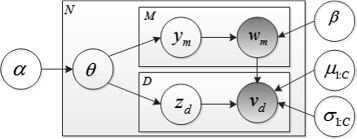

  

  Illustration of csGM-LDA.

• 2. For each associated tag $w_{m} \in {\mathcal W}=\{ 1,\cdots,C\},m=1,\cdots,M$

  • (a) Draw a topic assignment, $y_{m} \sim P_{Y|\Pi } (y_{m} |\theta),y_{m} \in {\mathcal T}_{y} =\{ 1,\cdots,K\}$

  • (b) Draw a tag, $w_{m} \sim P_{W|Y} (w_{m} |y_{m} ;\beta),w_{m} \in {\mathcal W}=\{ 1,\cdots,C\}$

• 3. For each visual word v _d ,d=1,⋯,D

  • (a) Draw a topic assignment, $z_{d} \sim P_{Z|\Pi } (z_{d} |\theta),z_{d} \in {\mathcal T}_{z} =\{ 1,\cdots,K\}$

  • (b) Draw a visual description, $v_{d} \sim P_{V|Z,W} (v_{d} |z_{d},w_{m} ;\mu _{w_{m}},\sigma _{w_{m}})\phantom {\dot {i}\!}$

Similar to the earlier LDA extensions, P _Π (·) is a Dirichlet distribution on the topic simplex $\theta \in \mathbb {R}^{K}$with the parameter $\alpha \in \mathbb {R}^{K}$, P _Y|Π (·) and P _Z|Π (·) are two multinomial distributions over the topic simplex θ, P _W|Y (·) is a categorical distribution over a topic y _m with the parameter $\beta \in \mathbb {R}^{K\times C}$ where β(k,c)=p(w _m =c|y _m =k), and P _V|Z,W (·) is a Gaussian distribution over a topic z _d with the class-dependent parameters $\left \{\mu _{w_{m}} (z_{d},d),\sigma _{w_{m}} (z_{d},d)|\mu _{w_{m}},\sigma _{w_{m}} \in \mathbb {R}^{K\times D} \right \}$. In this way, semantic topics generate tags or classes for images with each defining a prior distribution in visual topic space. Taking Bayesian rules, the joint distribution of {θ,y _m ,w _m ,z _d ,v _d } for each image is given by:

$$ \begin{array}{l} {P_{\Pi,Y,W,Z,V} (\theta,y_{m},w_{m},z_{d},v_{d} |\alpha,\beta,\mu_{w_{m}},\sigma_{w_{m}})= }\\ {P_{\Pi} (\theta |\alpha)P_{Y|\Pi} (y_{m} |\theta)P_{W|Y} (w_{m} |y_{m},\beta)P_{Z|\Pi} (z_{d} |\theta)}\\{P_{V|Z,W} (v_{d} |z_{d},\mu_{w_{m}},\sigma_{w_{m}}) } \end{array} $$

((12))

The modeling problem is then to maximize the log likelihood of the following marginal function:

$$ \begin{array}{l} {P_{W,V} (W,V|\alpha,\beta,\mu_{1:C},\sigma_{1:C})=} {\int_{\theta_{n} }\prod\limits_{n=1}^{N}\prod\limits_{m=1}^{M}\prod\limits_{d=1}^{D}\sum\limits_{y_{nm} }\sum\limits_{z_{nd} }}\\{P_{\Pi,Y,W,Z,V} (\theta_{n},y_{nm},w_{nm},z_{nd},v_{nd} |\alpha,\beta,\mu_{w_{nm}},\sigma_{w_{nm}}) d\theta_{n}} \end{array} $$

((13))

In csGM-LDA, the parameters {α,β,μ _1:C ,σ _1:C } are dataset-level parameters, assumed to be sampled once in the process of generating a set of images. The variables θ _n is an image-level variable, sampled once per image. The variables y _nm and w _nm are tag-level variables, sampled once for each annotated tag. And the variables z _nd and v _nd are structure-level variables, sampled once for each visual description. Structural models similar to that shown in Figure 1 are often studied in Bayesian statistical modeling, where they are referred to as conditionally independent hierarchical models. Indeed, as we discuss in the following subsection, we adopt the empirical Bayes approach to estimating parameters with a variational EM algorithm.

4.2 Parameter estimation via variational inference

In this section, we describe a convexity-based variational algorithm for parameter estimation. The basic idea of convexity-based variational inference is to make use of Jensen’s inequality to obtain an adjustable lower bound on the log likelihood [13]. Essentially, a family of lower bounds is usually indexed by a set of variational parameters. The variational parameters are chosen by an optimization procedure that attempts to find the tightest possible lower bound. In particular, the objective function in Equation 13 is usually intractable due to the couplings between θ _n and {β,μ _1:C ,σ _1:C } in the summation over latent topics. By dropping these edges and endowing the simplified graphical model with free variational parameters, we obtain a new family of distributions on the latent variables as seen in Figure 2. The variational distribution q(θ,Y,Z|η,ϕ,ζ) can be characterized by:

$$ {} {\small{\begin{aligned} q(\theta,Y,Z|\eta,\phi,\zeta)=\prod\limits_{n=1}^{N}q(\theta_{n} |\eta_{n})\prod\limits_{m=1}^{M}q(y_{nm} |\phi_{nm}) \prod\limits_{d=1}^{D}q(z_{nd} |\zeta_{nd}) \end{aligned}}} $$

((14))

Figure 2

The variational model for approximating csGM-LDA.

where {Y,Z} are the collections of latent topics, the Dirichlet parameter η _n , and the multinomial parameters {ϕ _nm ,ζ _nd } are the free variational parameters.

Having specified a simplified family of probability distributions, the next step is to set up an optimization problem that determines the values of the variational parameters:

$$ {\small{\begin{aligned} \left\{\eta^{*},\phi^{*},\zeta^{*} \right\}&=\arg \mathop{\min }\limits_{\left\{\eta,\phi,\zeta \right\}} D_{KL} \left(q(\theta,Y,Z|\eta,\phi,\zeta)\right.\\&\quad\left.||P_{\Pi,Y,Z} (\theta,Y,Z|W,V,\alpha,\beta,\mu_{1:C},\sigma_{1:C})\right) \end{aligned}}} $$

((15))

where D _KL (·) is the Kullback-Leibler (KL) divergence and {W,V} are the corresponding collections of their lowercase variables. To achieve this minimization, we begin with the expression of the true log-likelihood for an image-tag pair {W,V} by bounding the log likelihood of P _W,V (W,V|α,β,μ _1:C ,σ _1:C ) using the Jensen’s inequality:

$$ {} \begin{array}{l} {\log P_{W,V} (W,V|\alpha,\beta,\mu_{1:C},\sigma_{1:C}){\kern 1pt} \ge }\\ {E_{q} [\log P_{\Pi,Y,W,Z,V} (\theta,Y,W,Z,V|\alpha,\beta,\mu_{1:C},\sigma_{1:C})]}\\{-E_{q} [\log q(\theta,Y,Z|\eta,\phi,\zeta)]} \end{array} $$

((16))

It can be easily verified that the difference between the two sides of the above inequation is the KL divergence that provided in Equation 15. Let ${\mathcal L}(\eta,\phi,\zeta ;\alpha,\beta,\mu _{1:C},\sigma _{1:C})$ denote the right-hand side of the inequation, we have:

$$ {} {\small{\begin{aligned} \begin{array}{l} {\log P_{W,V} (W,V|\alpha,\beta,\mu_{1:C},\sigma_{1:C})=\mathcal{L}(\eta,\phi,\zeta ;\alpha,\beta,\mu_{1:C},\sigma_{1:C})+ }\\ {D_{KL} \left(q(\theta,Y,Z|\eta,\phi,\zeta)||P_{\Pi,Y,Z} (\theta,Y,Z|W,V,\alpha,\beta,\mu_{1:C},\sigma_{1:C})\right) } \end{array} \end{aligned}}} $$

((17))

This shows that maximizing the lower bound $\mathcal {L}(\eta,\phi,\zeta ;\alpha,\beta,\mu _{1:C},\sigma _{1:C})$ with respect to {η,ϕ,ζ} is equivalent to minimizing the above KL divergence. As seen in the Appendix, we obtain pair of updates:

$$ {} \left\{ \begin{array}{l} {\phi_{nm} (k)\propto \beta (k,w_{nm})\exp \left(\Psi (\eta_{n} (k))-\Psi \left(\sum_{j=1}^{K}\eta_{n} (j) \right)\right)} \\ {\zeta_{nd} (k)\propto \left(\prod\limits_{m=1}^{M}P_{V|Z,W} (v_{nd} |k,\mu_{w_{nm} },\sigma_{w_{nm} }) \right)}\\ {\quad\exp \left(\Psi (\eta_{n} (k))-\Psi \left(\sum\limits_{j=1}^{K}\eta_{n} (j) \right)\right)} \\ {\eta_{n} (k)=\alpha (k)+\sum_{m=1}^{M}\phi_{nm} (k) +\sum_{d=1}^{D}\zeta_{nd} (k) } \end{array} \right. $$

((18))

Based on the above variational inference, parameter estimation with respect to {α,β,μ _1:C ,σ _1:C } yields the following EM algorithm:

• 1. E-step: For each image, find the optimizing values of the variational parameters {η,ϕ,ζ}.

• 2. M-step: Maximize the resulting lower bound ${\mathcal L}(\eta,\phi,\zeta ;\alpha,\beta,\mu _{1:C},\sigma _{1:C})$on the log likelihood of P _W,V (W,V|α,β,μ _1:C ,σ _1:C ) with respect to the model parameters {α,β,μ _1:C ,σ _1:C }.

The update in the M-step corresponds to finding maximum likelihood estimates with expected sufficient statistics for each image under the approximate posterior which is computed by the variational parameters. Thus, we can also maximize the lower bound $\mathcal {L}(\eta,\phi,\zeta ;\alpha,\beta,\mu _{1:C},\sigma _{1:C})$ with respect to the parameters {α,β,μ _1:C ,σ _1:C }. In Appendix, we show that the update in the M-step for the Dirichlet parameter α can be implemented with an efficient Newton-Raphson method. The parameters {β,μ _1:C ,σ _1:C } can be obtained as:

$$ \left\{ \begin{array}{l} {\beta (k,c)\propto \sum_{n=1}^{N}\sum_{m=1}^{M}\phi_{nm} (k)\delta (c,w_{nm})} \\ {\mu_{c} (k,d)=\frac{\sum_{n=1}^{N}\sum_{m=1}^{M}\zeta_{nd} (k)\delta (c,w_{nm})v_{nd} }{\sum_{n=1}^{N}\sum_{m=1}^{M}\zeta_{nd} (k)\delta (c,w_{nm})} } \\ {{\sigma_{c}^{2}} (k,d)=\frac{\sum_{n=1}^{N}\sum_{m=1}^{M}\zeta_{nd} (k)\delta (c,w_{nm})\left(v_{nd} -\mu_{c} (k,d)\right)^{2} }{\sum_{n=1}^{N}\sum_{m=1}^{M}\zeta_{nd} (k)\delta (c,w_{nm})} } \end{array}\right. $$

((19))

We summarize the parameter estimation algorithm in Algorithm 2. This is a standard EM process, and the lower bound $\mathcal {L}(\eta,\phi,\zeta ;\alpha,\beta,\mu _{1:C},\sigma _{1:C})$ is a concave function. Therefore, Algorithm 2 is convergent. From the pseudo code, it is clear that each iteration of the E-step for csGM-LDA requires $\mathcal {O}(NMDK)$ operations. Empirically, we find that the number of iterations in this step is in proportion to the number of tags and the dimensionality of visual features. Parameter estimation in M-step for {β,μ _1:C ,σ _1:C } requires $\mathcal {O}(NCMDK)$ operations. And the number of iterations required for the Newton-Raphson method is linear to the dimensionality of α. Therefore, each EM iteration yields a total number of operations roughly on $\mathcal {O}\left (NM\left (C+M+D\right)DK\right)$. The number of iterations for the EM algorithm is mainly determined by the number of involved parameters, which is in proportion to C(1+D)K. Thus, the complexity for building the proposed model is about $\mathcal {O}\left (NCM\left (C+M+D\right)D^{2} K^{2} \right)$. When coping with large-scale data (i.e., N≫K,C,D), the complexity of our modeling system is approximately linear to the number of images, which is much effective by comparing with the typical quadratic annotation models (e.g., pLSA [13] that requires $\mathcal {O}\left (N^{2} KC\right)$ operations, GM-pLSA [27] that yields the number of operations roughly on $\mathcal {O}\left (N^{2} K^{2} C\right)$, and so on).

4.3 A unified framework for image annotation

The unified framework is illustrated in Figure 3. Laplacian regularized uncorrelated tensor representation is first performed on the whole dataset. Then, both the semantic and the visual modalities are incorporated into building the proposed model. To annotate a new image, we first get the corresponding core tensor and then predict potential tags with Bayesian inference.

Figure 3

Illustration of the proposed framework for image annotation.

Given an observed visual image, our goal for image annotation is to estimate the posterior distribution of the annotated tags. Taking Bayesian rules, we can infer their posterior probability by:

$$ {} {\footnotesize{\begin{aligned} \begin{array}{l} {P_{W|V} (w|v_{1:D},\alpha,\beta,\mu_{w},\sigma_{w})=\frac{P_{W,V} (w,v_{1:D} |\alpha,\beta,\mu_{w},\sigma_{w})}{P_{V} (v_{1:D} |\alpha,\beta,\mu_{w},\sigma_{w})}} \\ {=\frac{\int_{\theta }P_{\Pi} (\theta |\alpha)\left(\sum_{y}P_{Y|\Pi} (y|\theta)P_{W|Y} (w|y,\beta) \right)\left(\sum_{z_{d} }P_{Z|\Pi} (z_{d} |\theta)P_{V|Z,W} (v_{d} |z_{d},\mu_{w} (z_{d},d),\sigma_{w} (z_{d},d)) \right)d\theta }{\int_{\theta }P_{\Pi} (\theta |\alpha)\left(\sum_{z_{d} }P_{Z|\Pi} (z_{d} |\theta)P_{V|Z,W} (v_{d} |z_{d},\mu_{w} (z_{d},d),\sigma_{w} (z_{d},d)) \right)d\theta} } \end{array} \end{aligned}}} $$

((20))

For simplicity, we employ Monte Carlo inference [35] to approximate the integral of θ. To get the above probability, we first generate samples {θ ^s,s=1,⋯,S} from the posterior θ ^s∼P _Π (θ|α). Then, the tags’ probability can be rewritten by:

$$ {} {\small{\begin{array}{l} {P_{W|V} (w|v_{1:D},\alpha,\beta,\mu_{w},\sigma_{w})\approx}\\ {\frac{\sum_{s=1}^{S}\left(\sum_{y}P_{Y|\Pi} (y|\theta^{s})P_{W|Y} (w|y,\beta) \right)\left(\sum_{z_{d} }P_{Z|\Pi} (z_{d} |\theta^{s})P_{V|Z,W} (v_{d} |z_{d},\mu_{w},\sigma_{w}) \right) }{\sum_{s=1}^{S}\sum_{z_{d} }P_{Z|\Pi} (z_{d} |\theta^{s})P_{V|Z,W} (v_{d} |z_{d},\mu_{w} (z_{d},d),\sigma_{w} (z_{d},d))} } \end{array}}} $$

((21))

5 Experiments

To evaluate the performance of our annotation framework, we set up several quantitative experiments. First, we investigate the effects of the setting parameters by conducting cross validation to select the best parameters for our proposed model. Then, we give a comparison of different image representations and validate the effectiveness of our representation method. Finally, we evaluate the proposed method on two benchmark datasets and report the results over state of the art.

5.1 Datasets and representations

We evaluate the proposed framework on two well-known benchmarks: Corel-5K [36] and ESP-Game [37]. The details of the two image datasets are shown in Table 2. The training percentage of each dataset is set as 80%, a validation set occupies 10% of the total images, and the remainder is the test set.

Table 2 Statistics of two image datasets

To get a reasonable size that keeps the images from serious deterioration for our representation method, we fix the size of images in Corel-5K and ESP-Game as 128×192 and 225×169, respectively. The vectorization of the core tensor constituting the D-dimensional Laplacian regularized uncorrelated tensorial vector (LGUTV) can be viewed as an image descriptor, with each item corresponding to an uncorrelated elementary multilinear projection. In our experiment, the dimensionality of LGUTV is fixed as 128 for each group in both the two datasets. We further divide the Corel-5K and ESP-Game into five and ten groups by graph shift [34], resulting in a 640-dimensional vector and a 1,280-dimensional vector for these two datasets, respectively. In addition, we compare the proposed representation method with several common representation methods, i.e., the quantified color histograms with 16 bins in each color channel for RGB, LAB, HSV representations (C-HIST), the quantified SIFT features both extracted densely on a multiscale grid (D-SIFT) or for Harris-Laplacian interest points (H-SIFT) [3], local binary patterns (LBP) [38], and CPAM [4]. To get a proper evaluation of these image descriptors, we set their dimensions equal to that of LGUTV.

5.2 Evaluation criteria and baselines

The performance of image annotation is evaluated by comparing the automatically generated tags for the test set with the human-produced ground truth. In this paper, we give the following two measures for annotation evaluation. Firstly, F ₁ score is measured by computing precision (Prec) and recall (Rec) for fixed annotation length with the five most relevant tags.

$$ F_{1} =\frac{2\times Prec \times Rec}{Prec+Rec} $$

((22))

Note that each image is forced to be annotated with five tags, although the image might have fewer or more tags in the ground truth. Therefore, even if a model predicts all ground truth tags with a significantly higher probability than other tags, we will not measure perfect precision and recall. Thus, we also measure the precision at different levels of the recall for assessing the general annotation performance. The mean average precision (mAP) [13] over tags are found by computing for each tag the average of precisions measured after each relevant image is retrieved.

$$ mAP=\frac{1}{N_{q}} \sum\limits_{q=1}^{N_{q} }{\sum\limits_{i\in rel(q)} \text{Prec}(i) \left/ \left|rel(q)\right|\right.} $$

((23))

where Prec(i) is the precision of the correctly retrieved images at rank i in the ranking results of a query q, r e l(q) is the set of relevant images for this query, and N _q is the number of all queries.

For all images in the two standard datasets, our methods are compared with several most relevant and state-of-the-art methods, including TagProp [3], pLSA [13], GM-pLSA [27], GM-LDA [29], Corr-LDA [29], topic regression multimodal latent Dirichlet allocation (tr-mmLDA) [30], and css-LDA [16].

5.3 Investigate the impact of the setting parameters

We first investigate the neighborhood size K _NN for the graph construction and the tradeoff parameter λ for evaluating the effectiveness of Laplacian regularization. These two parameters reflect different facets of data construction; we joint discuss the sensitivity of these two parameters. As seen in Figure 4, we measure the F ₁ scores for different parameters by setting the number of latent topics equal to the number of tags. Then, we choose to set the two parameters as the most promising for the two datasets in the following experiments, which are K _NN =10,λ=0.1 for Corel-5K and K _NN =15,λ=0.1 for ESP-Game, respectively. Besides, we observe that Laplacian regularization can achieve a more effective representation for better semantic learning by comparing the case that λ≠0 with the case that λ=0.

Figure 4

Investigation of the neighborhood size and the tradeoff parameter. F ₁ score is measured to evaluate the performance of csGM-LDA by varying the two parameters on (a) Corel-5K and (b) ESP-Game.

Regarding topic models, they require the number of latent topics (i.e.,K) to be estimated, as this hyper parameter defines the capacity of the model. We analyze the parameter with a cross validation scheme. As seen in Figure 5, the improvement of annotation performance grows much slowly when the number of latent topics arrives at 100 for both the two datasets. When this number increases over the total number of tag vocabularies, csGM-LDA might suffer from the overfitting problem. For example, the measures of F ₁ score and mAP in both Figure 5a,b decrease when the number of latent topics is larger than 300. In the following experiments, we set the parameter as K=300, which achieves the best performance for both the two datasets.

Figure 5

Investigation of the number of latent topics. The performance of csGM-LDA is evaluated by taking different number of latent topics in terms of F ₁ score and mAP on (a) Corel-5K and (b) ESP-Game.

5.4 Evaluation of different image representations

In this paper, we argue that traditional vector-based image representations ignore high-order characteristics in image space, and thus, we combine unsupervised TSL and Laplacian regularization for achieving a more discriminative descriptor, i.e., LGUTV. To evaluate its effectiveness, we compare this descriptor with several state-of-the-art image descriptors on the two datasets by measuring F ₁ Scores for the results of csGM-LDA. As seen in Figure 6, the performance of modeling csGM-LDA with LGUTV achieves the best performance by comparing with others on both the two datasets, confirming that tensor representation is most likely to provide a discriminative descriptor for recognizing the complex visual scenes.

Figure 6

Annotation performance of csGM-LDA with different image representations.

5.5 Comparison with existing methods

In this section, we perform the annotation tasks on both the Corel-5K and ESP-Game datasets by comparing the proposed method with others. In Table 3, we report the performance by measuring both F ₁ score and mAP for different methods based on LGUTV. On both two datasets, we observe that class-specific methods (e.g., TagProp, css-LDA, and csGM-LDA) obviously perform better than others. This is consistent with the analysis in the introduction since the generative domains of the complex visual world are much hard to describe. In addition, the measures for ESP-Game are consistently lower than that for Corel-5K because the retrieval tasks on which these measures are now computed are more challenging: an average of nearly 2,000 images for testing (versus 500 images) are ranked. The proposed method achieves much more improvement on the ESP-Game dataset by comparing with a bit improvement on the Corel-5K dataset, demonstrating its effectiveness of modeling the large-scale dataset. For all the test sets, our proposed method performs best, and the instantiations of csGM-LDA and css-LDA clearly outperform others. We further compare the time required for training of different LDA models on ESP-Game and Corel-5K on a Intel Core i5-2410M CPU 2.30 GHz processor. Figure 7 gives the results. We observe that csGM-LDA is much faster than css-LDA. The reason is probably that the number of parameters in css-LDA is much larger than that of csGM-LDA. All the above results show the efficiency of our method.

Table 3 Comparison of different methods on both Corel-5K and ESP-Game

Figure 7

Time complexity of different LDA models on (a) Corel-5K and (b) ESP-Game.

6 Conclusions

In this paper, we propose a novel model, denoted as csGM-LDA, based on Laplacian regularized uncorrelated tensor representation for image annotation. The proposed annotation possesses two characteristics, namely: 1) images are represented by a set of uncorrelated tensorial descriptions and 2) class-specific information is integrated into semantic learning with the extension of the standard LDA model. The entire problem is formulated within the proposed framework, and csGM-LDA is presented to bridge the semantic gap between image contents and annotated tags. The experimental results demonstrate the effectiveness of our proposed method. Following the research on this line, we will further exploit region-based tensorial features for discriminative image representation and discuss the correlation of the class-specific information in a hierarchical LDA formalism.

7 Appendix

To maximize the lower bound in the E-Step that described in Section 4, we begin by expanding it with the factorizations of P _Π,Y,W,Z,V (θ,Y,W,Z,V|α,β,μ _1:C ,σ _1:C ) and q(θ,Y,Z|η,ϕ,ζ):

$${\small{\begin{array}{l} {{\mathcal L}(\eta,\phi,\zeta ;\alpha,\beta,\mu_{1:C},\sigma_{1:C})=E_{q} [\log P_{\Pi} (\theta |\alpha)]}\\{+E_{q} [\log P_{Y|\Pi} (Y|\theta)]+} {E_{q} [\log P_{W|Y} (W|Y,\beta)]}\\{+E_{q} [\log P_{Z} (Z|\theta)]+E_{q} [\log P_{V|Z,W} (V|Z,W,\mu_{1:C},\sigma_{1:C})]} \\ { -E_{q} [\log q(\theta |\eta)]-E_{q} [\log q(Y|\phi)]-E_{q} [\log q(Z|\zeta)]} \end{array}}} $$

We unfold each item, and obtain:

$$\begin{array}{*{20}l} P_{\Pi} (\theta |\alpha)&=\frac{\Gamma (\sum_{k}\alpha (k))}{\prod_{k}\Gamma (\alpha (k))} \prod\limits_{k}\theta (k)^{\alpha (k)-1},\\ P_{Y|\Pi} (y_{m} |\theta)&=\theta (y_{m}) \end{array} $$

$$P_{Z|\Pi} (z_{d} |\theta)=\theta (z_{d}),P_{W|Y} (w_{m} |y_{m},\beta)=\beta (y_{m},w_{m}) $$

$$\begin{array}{*{20}l} &P_{V|Z,W} (v_{d} |z_{d},\mu_{w_{m}},\sigma_{w_{m}})=\frac{1}{\sqrt{2\pi} \sigma_{w_{m}} (z_{d},d)}\\ &\quad\times \exp \left(-\frac{(v_{d} -\mu_{w_{m}} (z_{d},d))^{2} }{2\sigma_{w_{m} }^{2} (z_{d},d)} \right) \end{array} $$

To evaluate $\mathcal {L}(\eta,\phi,\zeta ;\alpha,\beta,\mu _{1:C},\sigma _{1:C})$, we should measure E _q (logθ). We find that the sufficient statistic in defining P _Π (θ|α) is logθ(k). Since the derivative of the log normalization factor with respect to the parameter is equal to the expectation of the sufficient statistic, we obtain:

$$E_{q} [\log \theta (k)]=\Psi (\eta (k))-\Psi \left(\sum_{k=1}^{K}\eta (k) \right) $$

where Ψ(·) is the first derivative of logΓ(·). Thus, we expand $\mathcal {L}(\eta,\phi,\zeta ;\alpha,\beta,\mu _{1:C},\sigma _{1:C})$ as:

$${} {\small{\begin{array}{l} {{\mathcal L}(\eta,\phi,\zeta ;\alpha,\beta,\mu_{1:C},\sigma_{1:C})= }\\ {\sum_{n=1}^{N}\left(\log \Gamma \left(\sum_{k=1}^{K}\alpha (k) \right)-\sum_{k=1}^{K}\log \Gamma (\alpha (k))\right. }\\{\left.+\sum_{k=1}^{K}\left(\alpha (k)-1\right)E[\log \theta_{n} (k)|\eta_{n} ] \right) } \\ +{\sum_{n=1}^{N}\sum_{m=1}^{M}\sum_{k=1}^{K}\phi_{nm} (k)E[\log \theta_{n} (k)|\eta_{n} ] }\\{+\sum_{n=1}^{N}\sum_{m=1}^{M}\sum_{k=1}^{K}\phi_{nm} (k)\log \beta (k,w_{nm}) } \\ +{\sum_{n=1}^{N}\!\sum_{d=1}^{D}\!\sum_{k=1}^{K}\zeta_{nd} (k)E[\log \theta_{n} (k)|\eta_{n} ] }\\ +{\sum_{n=1}^{N}\!\sum_{m=1}^{M}\!\sum_{d=1}^{D}\!\sum_{k=1}^{K}\!\zeta_{nd} (k)\log P_{V|Z,W} (v_{nd} |k,\mu_{w_{nm}},\sigma_{w_{nm} }) } \\ -{\sum_{n=1}^{N}\left(\log \Gamma (\sum_{k=1}^{K}\eta_{n} (k))+\sum_{k=1}^{K}\log \Gamma (\eta_{n} (k)) \right.}\\{\left.-\sum_{k=1}^{K}\left(\eta_{n} (k)-1\right)E[\log \theta_{n} (k)|\eta_{n} ] \right) } \\ -{\sum_{n=1}^{N}\sum_{m=1}^{M}\sum_{k=1}^{K}\phi_{nm} (k)\log \phi_{nm} (k) }\\{-\sum_{n=1}^{N}\sum_{d=1}^{D}\sum_{k=1}^{K}\zeta_{nd} (k)\log \zeta_{nd} (k) } \end{array}}} $$

In the E-Step, we first maximize the above function with respect to ϕ _nm (k). Observing that this is a constrained maximization since $\sum _{k=1}^{K}\phi _{\textit {nm}} (k) =1$, we first take the corresponding derivative:

$$\begin{array}{*{20}l}{} \frac{\partial \mathcal{L}}{\partial \phi_{nm} (k)} &=\Psi (\eta_{n} (k))-\Psi \left(\sum\limits_{j=1}^{K}\eta_{n} (j) \right)+\log \beta (k,w_{nm})\\&\quad-\log \phi_{nm} (k)-1 \end{array} $$

Adding Lagrange multipliers to and setting the derivative of the summation to zero yields the maximizing value of the variational parameter ϕ _nm (k):

$${} \phi_{nm} (k)\propto \beta (k,w_{nm})\exp \left(\Psi (\eta_{n} (k))-\Psi \left(\sum\limits_{j=1}^{K}\eta_{n} (j)\right)\right) $$

Similarly, we can obtain the variational parameter ζ _nd (k) as follows:

$$\begin{array}{*{20}l} \zeta_{nd} (k)&\propto \left(\prod\limits_{m=1}^{M}P_{V|Z,W} (v_{nd} |k,\mu_{w_{nm} },\sigma_{w_{nm}} \right)\\&\quad\times\exp \left(\Psi (\eta_{n} (k))-\Psi \left(\sum\limits_{j=1}^{K}\eta_{n} (j)\right)\right) \end{array} $$

Next, we maximize with respect to η _n (k). Taking the corresponding derivative, we obtain:

$${\small{\begin{array}{l} {\frac{\partial \mathcal{L}}{\partial \eta_{n} (k)} =\Psi '(\eta_{n} (k))\left(\vphantom{\sum_{m=1}^{M}\phi_{nm}}\alpha (k)-\eta_{n} (k)\right.}\\{{\kern6pc} \left.+\sum_{m=1}^{M}\phi_{nm} (k) +\sum_{d=1}^{D}\zeta_{nd} (k) \right)} \\ { -\sum_{k=1}^{K}\Psi '\left(\sum_{j=1}^{K}\eta_{n} (j) \right){\left(\left(\vphantom{\sum_{d=1}^{D}\zeta_{nd}}\alpha (k)-\eta_{n} (k)\right.\right.}}\\ {\left.\left.+\sum_{m=1}^{M_{n} }\phi_{nm} (k) +\sum_{d=1}^{D}\zeta_{nd} (k) \right)\right) } \end{array}}} $$

Setting this equation to zero yields a maximum at:

$$\eta_{n} (k)=\alpha (k)+\sum\limits_{m=1}^{M}\phi_{nm} (k) +\sum\limits_{d=1}^{D}\zeta_{nd} (k) $$

In the M-Step, we also maximize the resulting lower bound $\mathcal {L}(\eta,\phi,\zeta ;\alpha,\beta,\mu _{1:C},\sigma _{1:C})$ with respect to the model parameters {α,β,μ _1:C ,σ _1:C }. To estimate the Dirichlet parameter α, we first get the derivatives as:

$$\begin{array}{*{20}l} \frac{\partial \mathcal{L}}{\partial \alpha (k)} &=\sum\limits_{n=1}^{N}\left(\Psi \left(\sum\limits_{j=1}^{K}\alpha (j) \right)-\Psi (\alpha (k))\right.\\ &\quad\left.+\left(\Psi (\eta_{n} (k))-\Psi \left(\sum\limits_{j=1}^{K}\eta_{n} (j) \right)\right)\right) \end{array} $$

This derivative depends on α(j),for j≠k, and we therefore must use an iterative method to find the maximal α. In particular, we can invoke the Newton-Raphson method with the update:

$$\begin{array}{l}{} {\alpha^{(i+1)} (k)=\alpha^{(i)} (k)- }\\ {} {{\left(\frac{\partial {\mathcal L}}{\partial \alpha^{(i)} (k)} -\frac{\sum_{j=1}^{K}{\frac{\partial {\mathcal L}}{\partial \alpha^{(i)} (j)} \left/ \left(N\Psi '(\alpha^{(i)} (j))\right)\right.}}{{1\left/ \left(N\Psi '\left(\sum_{j=1}^{K}\alpha^{(i)} (j) \right)\right)\right.} +\sum_{j=1}^{K}{1\left/ \left(N\Psi '(\alpha^{(i)} (j))\right)\right.}} \right)\left/\vphantom{\sum_{j=1}^{K}{1\left/ \left(N\Psi '(\alpha^{(i)} (j))\right)\right.}}\right.}}\\ {} {{ \left(N\Psi '(\alpha^{(i)} (k))\right)}} \end{array} $$

To maximize $\mathcal {L}(\eta,\phi,\zeta ;\alpha,\beta,\mu _{1:C},\sigma _{1:C})$ with respect to β, we add Lagrange multipliers and set the derivative of the summation to zero, we can obtain:

$$\beta (k,c)\propto \sum\limits_{n=1}^{N}\sum\limits_{m=1}^{M}\phi_{nm} (k)\delta (c,w_{nm}) $$

As to {μ _1:C ,σ _1:C }, we set the corresponding derivatives of ${\mathcal L}(\eta,\phi,\zeta ;\alpha,\beta,\mu _{1:C},\sigma _{1:C})$ to zero and can exactly obtain:

$${} \mu_{c} (k,d)=\frac{\sum_{n=1}^{N}\sum_{m=1}^{M}\zeta_{nd} (k)\delta (c,w_{nm})v_{nd} }{\sum_{n=1}^{N}\sum_{m=1}^{M}\zeta_{nd} (k)\delta (c,w_{nm})} $$

$${} {\sigma_{c}^{2}} (k,d)=\frac{\sum_{n=1}^{N}\sum_{m=1}^{M}\zeta_{nd} (k)\delta (c,w_{nm})\left(v_{nd} -\mu_{c} (k,d)\right)^{2} }{\sum_{n=1}^{N}\sum_{m=1}^{M}\zeta_{nd} (k)\delta (c,w_{nm}) } $$

References

H Ma, J Zhu, M-T Lyu, I King, Bridging the semantic gap between image contents and tags. IEEE Trans. Multimedia. 12(5), 462–473 (2010).
J Liu, M Li, Q Liu, H Lu, S Ma, Image annotation via graph learning. Pattern Recognit. 42, 218–228 (2009).
M Guillaumin, T Mensink, J Verbeek, C Schmid, in Proc. IEEE Conf. Comput. Vis. Recognit. Tagprop: Discriminative metric learning in nearest neighbor models for image auto-annotation, (2009), pp. 309–316.
N Zhou, W Cheung, G Qiu, X Xue, A hybrid probabilistic model for unified collaborative and content-based image tagging. IEEE Trans. Pattern Anal. Mach. Intell. 33(7), 1281–1294 (2011).
S Yan, D Xu, Q Yang, L Zhang, X Tang, H-J Zhang, in Proc. IEEE Conf. Comput. Vis. Recognit. Discriminant analysis with tensor representation, (2005), pp. 526–532.
Y Liu, Y Liu, S Zhong, K Chan, Tensor distance based multilinear globality preserving embedding: a unified tensor based dimensionality reduction framework for image and video classification. Expert Syst. Appl. 39, 10500–10511 (2012).
Z Zhou, M Zhang, in Proc. Adv. Neural Inf. Process. Syst. Multi-instance multi-label learning with application to scene classification, (2006), pp. 1609–1616.
B-K Bao, T Li, S Yan, Hidden-concept driven multilabel image annotation and label ranking. IEEE Trans. Multimedia. 14(1), 199–210 (2012).
G Mesnil, A Bordes, J Weston, G Chechik, Y Bengio, Learning semantic representations of objects and their parts. Mach Learn. 94(2), 281–301 (2014).
J Li, J Wang, Automatic linguistic indexing of pictures by a statistical modeling approach. IEEE Trans. Pattern Anal. Mach. Intell. 25(9), 1075–1088 (2003).
Q Mao, I-H Tsang, S Gao, Objective-guided image annotation. IEEE Trans. Image Process. 22(4), 1585–1597 (2013).
D Blei, A Ng, M Jordan, Latent dirichlet allocation. J. Mach. Learn. Res. 3, 993–1022 (2003).
F Monay, D Gatica-Perez, Modeling semantic aspects for cross-media image indexing. IEEE Trans. Pattern Anal. Mach. Intell. 29(10), 1802–1817 (2007).
D Blei, J McAuliffe, in Proc. Adv. Neural Inf. Process. Syst. Supervised topic models, (2008), pp. 121–128.
Q Guo, N Li, Y Yang, G Wu, in IEEE International Conference on Systems, Man, and Cybernetics. Supervised LDA for image annotation, (2011), pp. 471–476.
N Rasiwasia, N Vasconcelos, Latent Dirichlet allocation models for image classification. IEEE Trans. Pattern Anal. Mach. Intell. 35(11), 2665–2679 (2013).
S Yan, D Xu, Q Yang, L Zhang, X Tang, H-J Zhang, Multilinear discriminant analysis for face recognition. IEEE Trans. Image Process. 16(1), 212–220 (2007).
D Tao, X Li, X Wu, S Maybank, General tensor discriminant analysis and gabor features for gait recognition. IEEE Trans. Pattern Anal. Mach. Intell. 29(10), 1700–1715 (2007).
J Yang, D Zhang, A Frangi, J Yang, Two-dimensional PCA: a new approach to appearance-based face representation and recognition. IEEE Trans. Pattern Anal. Mach. Intell. 26(1), 131–137 (2004).
J Ye, R Janardan, Q Li, in Proc. ACM SIGKDD Int’l Conf. Knowledge Discovery and Data Mining. Gpca: An efficient dimension reduction scheme for image compression and retrieval, (2004), pp. 354–363.
H Lu, K Plataniotis, A Venetsanopoulos, MPCA: multilinear principal component analysis of tensor objects. IEEE Trans. Neural Netw. 19(1), 18–39 (2008).
H Lu, K Plataniotis, A Venetsanopoulos, Uncorrelated multilinear principal component analysis for unsupervised multilinear subspace learning. IEEE Trans. Neural Netw. 20(11), 1820–1836 (2009).
J Ye, Generalized low rank approximations of matrices. Mach. Learn. 16(1), 167–191 (2005).
M Vasilescu, D Terzopoulos. Eur. Conf. Comput. Vis, (2002), pp. 447–460.
D Xu, S Yan, L Zhang, S Lin, H-J Zhang, T Huang, Reconstruction and recognition of tensor-based objects with concurrent subspaces analysis. IEEE Trans. Circuits Syst. Video Technol. 18(1), 36–47 (2008).
B Zhou, F Zhang, L Peng, Compact representation for dynamic texture video coding using tensor method. IEEE Trans. Circuits Syst. Video Technol. 23(2), 280–288 (2013).
Z Li, Z Shi, X Liu, Z Shi, Modeling continuous visual features for semantic image annotation and retrieval. Pattern Recognit. Lett. 32, 516–523 (2011).
S Nikolopoulos, S Zafeiriou, I Patras, I Kompatsiaris, High-order pLSA for indexing tagged images. Signal Process. 93, 2212–2228 (2013).
D Blei, M Jordan, in Proc. 26nd Ann. Int’l ACM SIGIR Conf. Research and Development in Information Retrieval. Modeling annotated data, (2003), pp. 127–134.
D Putthividhya, H Attias, S Nagarajan, in Proc. IEEE Conf. Comput. Vis. Recognit. Topic regression multi-modal latent Dirichlet allocation for image annotation, (2010), pp. 3408–3415.
L Zhuang, H Gao, J Luo, Z Lin, Regularized semi-supervised latent Dirichlet allocation for visual concept learning. Neurocomputing. 119, 26–32 (2013).
H Lu, K Plataniotis, A Venetsanopoulos, A survey of multilinear subspace learning for tensor data. Pattern Recognit. 44, 1540–1551 (2011).
W-Y Ma, B Manjunath, Edgeflow: a technique for boundary detection and image segmentation. IEEE Trans. Image Process. 9(8), 1375–1388 (2000).
H Liu, S Yan, in International Conference on Machine Learning. Robust graph mode seeking by graph shift, (2010), pp. 671–6783.
K Murphy, Machine Learning: A Probabilistic Perspective (The MIT Press, 2012).
H Müller, S Marchand-Maillet, T Pun, in Proc. ACM Int’l Conf. Image and Video Retrieval. The truth about Corel evaluation in image retrieval, (2002), pp. 38–49.
L Ahn, L Dabbish, in Proc. ACM SIGCHI Conf. on Human Factors in Computing Systems. Labeling images with a computer game, (2004), pp. 354–363.
T Ahonen, A Hadid, M Pietikainen, Face description with local binary patterns: application to face recognition. Mach. Learn. 28(12), 2037–2041 (2006).
Acknowledgement
This research was conducted with the support of National Natural Science Foundation of China (Grant No. 61271439).
Author information
Authors and Affiliations
Corresponding author
Additional information
Competing interests
The authors declare that they have no competing interests.
Rights and permissions
Open Access This article is distributed under the terms of the Creative Commons Attribution 4.0 International License (https://creativecommons.org/licenses/by/4.0), which permits use, duplication, adaptation, distribution, and reproduction in any medium or format, as long as you give appropriate credit to the original author(s) and the source, provide a link to the Creative Commons license, and indicate if changes were made.
About this article
Cite this article
Qian, Z., Zhong, P. & Wang, R. Class-specific Gaussian-multinomial latent Dirichlet allocation for image annotation. EURASIP J. Adv. Signal Process. 2015, 40 (2015). https://doi.org/10.1186/s13634-015-0224-z
Received:
Accepted:
Published:
DOI: https://doi.org/10.1186/s13634-015-0224-z