- Research Article
- Open access
- Published:
Robust and Accurate Curvature Estimation Using Adaptive Line Integrals
EURASIP Journal on Advances in Signal Processing volume 2010, Article number: 240309 (2010)
Abstract
The task of curvature estimation from discrete sampling points along a curve is investigated. A novel curvature estimation algorithm based on performing line integrals over an adaptive data window is proposed. The use of line integrals makes the proposed approach inherently robust to noise. Furthermore, the accuracy of curvature estimation is significantly improved by using wild bootstrapping to adaptively adjusting the data window for line integral. Compared to existing approaches, this new method promises enhanced performance, in terms of both robustness and accuracy, as well as low computation cost. A number of numerical examples using synthetic noisy and noiseless data clearly demonstrated the advantages of this proposed method over state-of-the-art curvature estimation algorithms.
1. Introduction
Curvature is a widely used invariant feature in pattern classification and computer vision applications. Examples include contour matching, contour segmentation, image registration, feature detection, object recognition, and so forth. Since curvature is defined by a function of higher-order derivatives of a given curve, the numerically estimated curvature feature is susceptible to noise and quantization error. Previously, a number of approaches such as curve/surface fitting [1–5], derivative of tangent angle [6, 7], and tensor of curvature [8–11] have been proposed with moderate effectiveness. However, an accurate and robust curvature estimation method is still very much desired.
Recently, the integral invariants [12–14] have begun to draw significant attention from the pattern recognition community due to their robustness to noise. These approaches have been shown as promising alternatives for extracting geometrical properties from discrete data. While curvature is just a special instance of invariant features under the rigid transformations (composition of rotations and translations), it is arguably the most widely used one in computer vision applications.
In this paper, we propose a novel curvature estimator based on evaluating line integrals over a curve. Since our method does not require derivative evaluations, it is inherently robust with respect to sampling and quantization noise. In contrast to the previous efforts, we are interested here in the line integral. It should be noted that the strategy presented by Pottmann et al. [14] can be trivially changed to compute curvature on curves. However, the resultant curvature estimate requires surface integrals taken over local neighborhoods. Compared with surface integral (also known as double integral), the line-integral formulation for curvature estimation has a reduced computational complexity in general. We will further discuss the complexity of numerical integration in Section 3.
Our method is also a significant improvement over the previously reported work [14] in terms of estimation accuracy. This is because the earlier work evaluates integrals over a user-defined, fixed-size window surrounding the point where curvature is to be evaluated. Depending on the sharpness of the curvature, the window size may be too large or too small. An over-sized window would dilute the distinct curvature feature by incorporating irrelevant points on the curve into the integral. An under-sized window, on the other hand, would be less robust to noise and quantization errors.
In this proposed curvature estimation algorithm, we evaluate line integrals over a window whose size is adaptively determined using the wild bootstrap procedure [15]. As such, the size of the data window will be commensurate to the sharpness of the curvature to be estimated, and the resulting accuracy is expected to be significantly improved. The performance advantage of this proposed adaptive window curvature estimation algorithm has been examined analytically, and has been validated using several numerical experiments.
The rest of this paper is organized as follows. Section 2 provides a brief review on the related work. In Section 3, the curvature estimation method based on line integrals is introduced. We subsequently formulate the problem of choosing an optimal window size and derive an adaptive curvature estimator in Section 4. In Section 5, we provide experimental results to show the robustness and accuracy of the proposed method. Comparisons with existing curvature estimation methods are also included. Finally, we make concluding remarks and discuss future works in Section 6.
2. Related Work
Due to the needs of many practical applications, extensive research has been conducted on the problem of curvature estimation. In a real-world application, data are often given in discrete values sampled from an object. Hence, one is required to estimate curvature or principal curvatures from discrete values. Flynn and Jain [4] report an empirical study on five curvature estimation methods available at that time. Their study's main conclusion is that the estimated curvatures are extremely sensitive to quantization noise and multiple smoothings are required to get stable estimates. Trucco and Fisher [16] have similar conclusion. Worring and Smeulders [7] identify five essentially different methods for measuring curvature on digital curves. By performing a theoretical analysis, they conclude that none of these methods is robust and applicable for all curve types. Magid et al. [17] provide a comparison of four different approaches for curvature estimation on triangular meshes. Their work manifests the best algorithm suited for estimating Gaussian and mean curvatures.
In the following sections, we will discuss different kinds of curvature estimation methods known in the literature. Also, we will review some related work in integral invariants and adaptive window selection.
2.1. Derivative of the Tangent Angle
The approaches based on the derivative of tangent can be found in [6, 18–20]. Given a point on a curve, the orientation of its tangent vector is first estimated and then curvature is calculated by Gaussian differential filtering. This kind of methods are preferable when computational efficiency is of primary concern. The problem associated with these approaches is that estimating tangent vector is highly noise-sensitive and thus the estimated curvature is unstable in real world applications.
2.2. Radius of the Osculating Circle
The definition of osculating circle leads to algorithms which fit a circular arc to discrete points [2, 3, 21]. The curvature is estimated by computing the reciprocal of the radius of an osculating circle. An experimental evaluation of this approach is presented in the classical paper by Worring and Smeulders [7]. The results reveal that reliable estimates can only be expected from arcs which are relatively large and of constant radius.
2.3. Local Surface Fitting
As the acquisition and use of 3D data become more widespread, a number of methods have been proposed for estimating principal curvatures on a surface. Principal curvatures provide unique view-point invariant shape descriptors. One way to estimate principal curvatures is to perform surface fitting. A local fitting function is constructed and then curvature can be calculated analytically from the fitting function. The popular fitting methods include paraboloid fitting [22–24] and quadratic fitting [1, 25–27]. Apart from these fitting techniques, other methods have been proposed, such as higher-order fitting [5, 28] and circular fitting [29, 30].Cazals and Pouget[5] perform a polynomial fitting and show that the estimated curvatures converge to the true ones in the case of a general smooth surface. A comparison of local surface geometry estimation methods can be found in [31].
The paper written by Flynn and Jain [4] reports an empirical evaluation on three commonly used fitting techniques. They conclude that reliable results cannot be obtained in the presence of noise and quantization error.
2.4. The Tensor of Curvature
The tensor of curvature has lately attracted some attention [8–11, 32]. It has been shown as a promising alternative for estimating principal curvatures and directions. This approach is first introduced by Taubin [8], followed by the algorithms which attempt to improve accuracy by tensor voting [9–11, 32]. Page et al. [9] present a voting method called normal voting for robust curvature estimation, which is similar to [10, 32]. Recently,Tong and Tang[11] propose a three-pass tensor voting algorithm with improved robustness and accuracy.
2.5. Integral Invariants
Recently, there is a trend on so-called integral invariants which reduce the noise-induced fluctuations by performing integrations [12, 13]. Such integral invariants possess many desirable properties for practical applications, such as locality (which preserves local variations of a shape), inherent robustness to noise (due to integration), and allowing multiresolution analysis (by specifying the interval of integration). In [14], the authors present an integration-based technique for computing principal curvatures and directions from a discrete surface. The proposed method is largely inspired by both Manay et al. [13] and Pottmann et al. [14], in which they use a convolution approach to calculate an integral. In this paper, we investigate avoiding the convolution with polynomial complexity by instead using the one with constant complexity.
2.6. Adaptive Window Selection
The curvature estimation algorithms mentioned above have the shortcoming of using a fixed window size. On one hand, if a large window is selected, some fine details on a shape will be smoothed out. On the other hand, if a small window is utilized, the effect of discretization and noise will be salient and the resultant estimate will have a large variance. To mitigate this fundamental difficulty in curvature estimation, a window size must be determined adaptively depending on local characteristics.
A number of publications concerning the issue of adaptive window selection have appeared in the last two decades [33–37]. In the dominant point detection algorithms [33, 35, 36], it is important to select a proper window for estimating curvature. Teh and Chin [33] use the ratio of perpendicular distance and the chord length to determine the size of a window.B. K. Ray and K. S. Ray[35] introduce a new measurement, namely,  -cosine, to decide a window adaptively based on some local properties of a curve. Wu [36] proposes a simple measurement which utilizes an adaptive bending value to select the optimal window.
Recently, the bootstrap methods [38] have been applied with great success to a variety of adaptive window selection problems. Foster and Zychaluk [37] present an algorithm for estimating biological transducer functions. They utilize a local fitting with bootstrap window selection to overcome the problems associated with traditional polynomial regression. Inspired by their work, we develop an adaptive curvature estimation algorithm based on the wild bootstrap method [15, 39]. We will elaborate the associated window selection algorithm in Section 4.
3. Curvature Estimation by Line Integrals
In this section, we introduce the approach for estimating curvature along a planar curve by using line integrals.
First, we briefly review some important results in differential geometry. Interested readers may refer to [40] for more details. Let  be an interval and
  be a curve parameterized by arc length
  . To proceed with local analysis, it is necessary to add the assumption that the derivative
  always exists. We interpret
  as the trajectory of a particle moving in a 2-dimensional space. The moving plane determined by the unit tangent and normal vectors,
  and
and  , is called the osculating plane at
  .
.
In analyzing the local properties of a point on a curve, it is convenient to work with the coordinate system associated with that point. Hence, one can write the equation of a curve, in the neighborhood of  , by using
  and
and  as a coordinate frame. In particular,
  is the
  -axis and
  is the
  -axis. The Taylor series expansion of the curve in the neighborhood of
  , denoted by
  , with respect to the local coordinate frame centered at
  , is given by

where  is the remainder. Since
  ,
,  , and
, and  is the curvature at
  , we obtain that
  , where
  denotes the curvature at
  . For a point on a curve, let
  denote a circle with center at that point and radius
  . Then, we can perform the line integral of an arbitrary function
  along
along  ,
,

where  and
and  is the arc length element; in other words,
  is the portion of the circle
  that is above
  . An example of a circle and the corresponding integral region
  is shown in Figure 1(a). The line integral
  can be approximated by

where  denotes the upper half of
  , that is,
 . In (3), we first perform line integral on the upper half of
  (the first term) and then subtract the line integrals on the portions of
  that are between
  and
and  -axis (the second and third terms). We utilize two straight lines to approximate the portions of
  bounded by
  and
and  -axis.

(a) For a point (the black square dot) on a curve  (the gray line), we draw a circle
  centered at that point. The integral region
  is denoted by red dashed line. It is convenient to write the equation of the curve, in the neighborhood of
  , using
  and
and  as a coordinate frame. (b) After obtaining
  and
and  , the line integrals can be easily computed. It does not matter which coordinate system we use for computing
  and
and  . One can always obtain a curvature estimate by performing eigenvalue decomposition.
Let  , the covariance matrix
  of the region
  is given by

where  and
and  denote the length and the barycenter of
  , respectively. Because the region
  is symmetric, the line integral
  is equal to zero for any odd function
  . Hence, we have
  and
and  . By using (3), we can then obtain

Therefore, the covariance matrix  can be approximated by

From (6), we can obtain the following relationship:

So, curvature  can be estimated by performing the principal component analysis on the region
  . In a real-world application, it does not matter which coordinate system is used for computing a covariance matrix. One can conduct the eigenvalue decomposition of
  and then obtain a curvature estimate. The procedure for curvature estimation is as follows.
-
(1)
Let
 be a point on a curve. We draw a circle with radius
  centered at
  . The intersections of the circle and the curve are denoted by
  and
and  . The angle between the vector
  and the
  -axis is denoted by
  . Similarly,
  denotes the angle between the vector
  and the
  -axis. An example is shown in Figure 1(b).
 -
(2)
Calculate the covariance matrix
 associated with point
  . Following directly from (4), we have
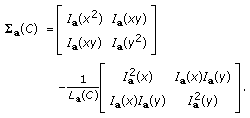 (8)
(8)It is straightforward to show that the line integrals can be calculated as follows:
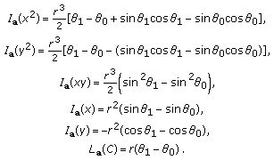 (9)
(9) -
(3)
The covariance matrix
 can be factored as
 (10)
(10)where
 contains the eigenvalues of
  and
and  contains the corresponding eigenvectors. Because
  is real and symmetric, the eigenvectors
  and
and  are orthogonal. Generally speaking, (10) shows the Singular Value Decomposition (SVD) and thus the diagonal elements of
  are also called the singular values of
  .
. -
(4)
The unit tangent at
 , denoted by
  , must be parallel to either
  or
or  . If the eigenvector parallel to
  were identified, one could compute curvature by using the corresponding eigenvalue (see (7)). Here, we choose the eigenvalue by comparing signs of inner products
  and
and  . If
. If  were parallel to
  , the signs of
  and
and  must be different. One can use either
  or
or  . Pseudocode for computing curvature utilizing
  is shown below.
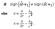 (11)
(11)
 be a point on a curve. We draw a circle with radius
  centered at
  . The intersections of the circle and the curve are denoted by
  and
and  . The angle between the vector
  and the
  -axis is denoted by
  . Similarly,
  denotes the angle between the vector
  and the
  -axis. An example is shown in Figure
  associated with point
  . Following directly from (4), we have

 can be factored as
 contains the eigenvalues of
  and
and  contains the corresponding eigenvectors. Because
  is real and symmetric, the eigenvectors
  and
and  are orthogonal. Generally speaking, (10) shows the Singular Value Decomposition (SVD) and thus the diagonal elements of
  are also called the singular values of
  .
. , denoted by
  , must be parallel to either
  or
or  . If the eigenvector parallel to
  were identified, one could compute curvature by using the corresponding eigenvalue (see (7)). Here, we choose the eigenvalue by comparing signs of inner products
  and
and  . If
. If  were parallel to
  , the signs of
  and
and  must be different. One can use either
  or
or  . Pseudocode for computing curvature utilizing
  is shown below.
Note that the numerical integration is typically computed by convolution in the previous work [13, 14]. For example, when evaluating the area integral invariant [13] of a particular point on a curve, the standard convolution algorithm has a quadratic computational complexity. With the help of the convolution theorem and the Fast Fourier Transform (FFT), the complexity of convolution can be significantly reduced [14]. However, the running time required by the FFT is  , where
  equals the number of sampling points in an integral region. Compared with the earlier methods [13, 14], the complexities of the integrals in (8) are constant and hence our method is computationally more efficient.
4. Adaptive Radius Selection
A critical issue in curvature estimation by line integrals lies in selecting an appropriate circle. The circle  must be large enough to include enough data points for reliable estimation, but small enough to avoid the effect of oversmoothing. For this reason, the radius of a circle must be selected adaptively, based on local shapes of a curve. In this section, we will first formulate the problem of selecting an optimal radius and then present an adaptive radius selection algorithm.
Intuitively, an optimal radius can be obtained by minimizing the difference between the estimated curvature  , based on the data within radius
  , to its true value
  . A common way to quantify the difference between
  and
and  is to compute the Mean Squared Error (MSE) as a function of
  , that is,

where  is the expectation (the value that could be obtained if the distribution of
  were available). However, the minimizer of
  cannot be found in practice since it involves an unknown value
  .
.
The bootstrap method [38], which has been extensively analyzed in the literature, provides an effective means for overcoming such a difficulty. In (12), one can simply replace the unknown value  with the estimate obtained from a given dataset, then replace the original estimate
  with the estimates computed from bootstrap datasets. Therefore, the optimal radius can be determined by

where the asterisks denote that the statistics are obtained from bootstrap samples.
The conceptual block diagram of the radius selection algorithm using bootstrap method is shown in Figure 2 and the detailed steps are described below.
-
(1)
Given a point
 on a curve, we draw an initial circle of radius
  .
. -
(2)
By using the estimator described in Section 3, the estimate
 is calculated from the neighboring points of
  within radius
  . In the rest of this paper, we will use
  to denote the neighboring points of
  within radius
  .
. -
(3)
The local shape around
 can be modeled by
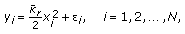 (14)
(14)where
 is called a modeling error or residual. Note that we use the moving plane described in Section 3 as our local coordinate system.
 -
(4)
Generate wild bootstrap residuals
 from a two-point distribution [15]:
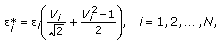 (15)
(15)where the
 's are independent standard normal random variables.
 -
(5)
The wild bootstrap samples
 are constructed by adding the bootstrap residuals
  :
: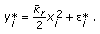 (16)
(16)We use
 to denote a wild bootstrap dataset.
 -
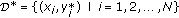
(6)
By repeating the third to the fifth steps, we can generate many wild bootstrap datasets, that is,
 . The larger the number of wild bootstrap datasets, the more satisfactory the estimate of a statistic will be.
 -
(7)
We can then obtain bootstrap estimates
 from the wild bootstrap datasets
  . The bootstrap estimate of the
  is given by
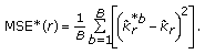 (17)
(17) -
(8)
The optimal radius is defined as the minimizer of (17), that is,
 (18)
(18)
 on a curve, we draw an initial circle of radius
  .
. is calculated from the neighboring points of
  within radius
  . In the rest of this paper, we will use
  to denote the neighboring points of
  within radius
  .
. can be modeled by
 is called a modeling error or residual. Note that we use the moving plane described in Section 3 as our local coordinate system.
 from a two-point distribution [
 's are independent standard normal random variables.
 are constructed by adding the bootstrap residuals
  :
:
 to denote a wild bootstrap dataset.
 . The larger the number of wild bootstrap datasets, the more satisfactory the estimate of a statistic will be.
 from the wild bootstrap datasets
  . The bootstrap estimate of the
  is given by


Block diagram of the radius selection algorithm using bootstrap method.
5. Experiments and Results
We conduct several experiments to evaluate the performance of the proposed adaptive curvature estimator. In Section 5.1, we demonstrate how the radius of the estimator changes with respect to local contour geometry. In Section 5.2, the experiments are conducted to verify whether the adaptivity provides an improved estimation accuracy. And, the robustness of the proposed method is experimentally validated in Section 5.3.
5.1. Qualitative Experiments
These experiments are intended to qualitatively verify the behavior of selecting an optimal radius. The curves  are utilized as test subjects in the experiments. The sampling points along a curve are generated by performing sampling uniformly along the
  -axis. The radius of the proposed adaptive curvature estimator ranges from
  to
to  with the step size of
  . Figure 3 shows the adaptively varying radii obtained by our method. We can see that the radius is relatively small near the point at
  and become larger as
  is increasing. This phenomenon corresponds to our expectation that a smaller radius should be chosen at a point with high curvature so that smoothing effect can be reduced. In a low-curvature area, a larger radius should be selected so that a more reliable estimate can be obtained. Since the behavior is in accordance with the favorable expectation, the remaining issue is whether the adaptively selected radius indeed improves estimation accuracy. In the following section, we will perform an experimental validation on this issue.

The proposed adaptive curvature estimator is applied to the curves depicted in (a), (c), and (e). The resultant radii of  are shown in (b), (d), and (f), respectively.
5.2. Quantitative Experiments
In the quantitative analysis, the curvature estimate obtained by adaptive radius is compared against the true curvature, and the estimate obtained by fixed radii. In Figure 4, it can be seen that the curvature estimator with a fixed undersize radius will be accurate at the peak but inaccurate in the flat regions. On the other hand, the curvature estimator with a fixed oversize radius will lead to over smoothing and hence be inaccurate at the peak. Therefore, it is desirable that the curvature estimator could adapt according to the input data. By adjusting the radius adaptively, we observe that the precision of curvature estimation is significantly improved. Figure 5 depicts the estimation errors of using fixed radii and adaptive radius. It is obvious that the estimation errors of the adaptive radius algorithm are much smaller than those of the fixed radius algorithm. In short, we have demonstrated that the estimation accuracy depends largely on the radius of  and it can be significantly improved by using adaptive radius.

True curvatures and estimated curvatures of the curves in (a), (c), and (e) are shown in (b), (d), and (f), respectively. The curvature estimates are obtained by an adaptive radius and fixed radii.

5.3. Sensitivity to Perturbations
In Section 3, the concept of curvature estimation via line integrals has been developed under an error-free assumption. However, in practical applications, perturbations in the input data can arise from many sources, such as roundoff errors or sensor noise. In this section, we will evaluate the robustness of the proposed curvature estimator and will compare it with existing approaches.
Before dealing with noisy data, we first consider noise-free cases. Two curves are utilized in our experiments. One is a sinusoidal curve which contains both positive and negative curvatures (see Figure 6(a)). The other one is a closed curve given by  (see Figure 8(a)). These continuous curves have been discretized by uniformly sampling in the angular variable and curvature is estimated at each sampling point.

(a) A sinusoidal waveform, (b) curvature estimate obtained by derivative of tangent, (c) curvature estimate obtained by Calabi et al.'s algorithm, (d) curvature estimate obtained by Taubin's algorithm, (e) curvature estimate obtained by line integrals, and (f) curvature estimate obtained by line integrals with adaptive radius. Notice that a dashed blue line denotes the true curvature.
Figures 6(b) and 8(b) give the curvature estimate obtained by the derivative of tangent [7]. The results obtained by Calabi et al.'s method [41] are shown in Figures 6(c) and 8(c). Both of these methods calculate a curvature estimate from three successive sampling points and thus can yield an excellent accuracy under a noise-free condition. However, this kind of approach cannot have reliable results under practical situations where perturbations are inevitable. By using another integral-based method [8], the curvature estimates calculated from the noisy shapes are shown in Figures 7(d) and 9(d). Similar to the proposed method with a fixed radius, this method can obtain reliable results from noisy data but has large estimation errors in high curvature regions.

Trial-to-trial variability in curvature estimates. The data consist of 10 trials. (a) sinusoidal waveforms with additive Gaussian noise, (b) curvature estimate obtained by derivative of tangent, (c) curvature estimate obtained by Calabi et al.'s algorithm, (d) curvature estimate obtained by Taubin's algorithm, (e) curvature estimate obtained by line integrals, and (f) curvature estimate obtained by line integrals with adaptive radius. Notice that these figures have different ranges in vertical coordinate because some methods yield noisy results. The true curvature is denoted by a dashed blue line.

(a) The closed curve
 , (b) curvature estimate obtained by derivative of tangent, (c) curvature estimate obtained by Calabi et al.'s algorithm, (d) curvature estimate obtained by Taubin's algorithm, (e) curvature estimate obtained by line integrals, and (f) curvature estimate obtained by line integrals with adaptive radius. Notice that a dashed blue line denotes the true curvature.

Trial-to-trial variability in curvature estimates. The data consist of 10 trials. (a) The closed curves  with additive Gaussian noise, (b) curvature estimate obtained by derivative of tangent, (c) curvature estimate obtained by Calabi et al.'s algorithm, (d) curvature estimate obtained by Taubin's algorithm, (e) curvature estimate obtained by line integrals, and (f) curvature estimate obtained by line integrals with adaptive radius. Notice that these figures have different ranges in vertical coordinate because some methods yield noisy results. The true curvature is denoted by a dashed blue line.
Compared with the above mentioned methods, the proposed curvature estimator with a fixed radius has larger estimation errors, especially in sharp regions (Figures 6(e) and 8(e)). This is an expected result because the circle  provides a smoothing effect on sharp corners. As one can see in Figures 6(f) and 8(f), the estimation accuracy is significantly improved once the radius of
  at each point is adaptively determined.
In the following experiments, we add noise to the original shapes and then perform curvature estimation on the noisy shapes. Figure 7 depicts the results of  trials. It is obvious that the proposed method, with or without adaptive radius, is able to obtain reasonable estimates while the derivative of tangent [7] and Calabi et al.'s algorithm [41] have significantly larger trial-to-trial variabilities. The same phenomenon is also observed in Figure 9. The results strongly suggest that sensitivity to perturbations is significantly reduced by using the proposed method. The proposed approach for curvature estimation is clearly a better choice if the input data are likely to be noisy.
6. Conclusions and Future Work
A novel curvature estimator, which achieves robustness to noise without sacrificing estimation accuracy, is presented in this paper. The novelty of the proposed method lies in performing line integrals on a circle. Because of performing integrations, we can avoid numerical differentiation which is a notoriously unstable process. Furthermore, instead of choosing a fixed radius for the circle, an optimal radius is determined at each point to minimize estimation error. We present extensive simulation results that demonstrate the effectiveness of our approach as compared with the recently proposed approaches [7, 8, 41]. Notice that we choose [8] for comparison because it is frequently used as a baseline algorithm in the literature. Although the estimator introduced by Taubin [8] is aiming for principal curvatures on surfaces, it can be trivially changed to compute curvature on curves.
An important issue for future research is to generalize the proposed framework to the estimation of principal curvature. To position our approach among others, we would also like to conduct a comparative study of more curvature estimation methods.
References
Besl PJ, Jain RC: Invariant surface characteristics for 3D object recognition in range images. Computer Vision, Graphics and Image Processing 1986, 33(1):33-80. 10.1016/0734-189X(86)90220-3
Landau UM: Estimation of a circular arc center and its radius. Computer Vision, Graphics and Image Processing 1987, 38(3):317-326. 10.1016/0734-189X(87)90116-2
Thomas SM, Chan YT: A simple approach for the estimation of circular arc center and its radius. Computer Vision, Graphics and Image Processing 1989, 45(3):362-370. 10.1016/0734-189X(89)90088-1
Flynn PJ, Jain AK: On reliable curvature estimation. Proceedings of the IEEE Conference on Computer Vision and Pattern Recognition, 1989 110-116.
Cazals F, Pouget M: Estimating differential quantities using polynomial fitting of osculating jets. Computer Aided Geometric Design 2005, 22(2):121-146. 10.1016/j.cagd.2004.09.004
Asada H, Brady M: The curvature primal sketch. IEEE Transactions on Pattern Analysis and Machine Intelligence 1986, 8(1):2-14.
Worring M, Smeulders AWM: Digital curvature estimation. CVGIP: Image Understanding 1993, 58(3):366-382. 10.1006/ciun.1993.1048
Taubin G: Estimating the tensor of curvature of a surface from a polyhedral approximation. Proceedings of the 5th International Conference on Computer Vision, June 1995 902-907.
Page DL, Koschan A, Sun Y, Paik J, Abidi MA: Robust crease detection and curvature estimation of piecewise smooth surfaces from triangle mesh approximations using normal voting. Proceedings of the IEEE Computer Society Conference on Computer Vision and Pattern Recognition, December 2001 1: 162-167.
Tang C-K, Medioni G: Curvature-augmented tensor voting for shape inference from noisy 3D data. IEEE Transactions on Pattern Analysis and Machine Intelligence 2002, 24(6):858-864. 10.1109/TPAMI.2002.1008395
Tong W-S, Tang C-K: Robust estimation of adaptive tensors of curvature by tensor voting. IEEE Transactions on Pattern Analysis and Machine Intelligence 2005, 27(3):434-449.
Hann CE, Hickman MS: Projective curvature and integral invariants. Acta Applicandae Mathematicae 2002, 74(2):177-193. 10.1023/A:1020617228313
Manay S, Cremers D, Hong B-W, Yezzi AJ Jr., Soatto S: Integral invariants for shape matching. IEEE Transactions on Pattern Analysis and Machine Intelligence 2006, 28(10):1602-1617.
Pottmann H, Wallner J, Yang Y-L, Lai Y-K, Hu S-M: Principal curvatures from the integral invariant viewpoint. Computer Aided Geometric Design 2007, 24(8-9):428-442. 10.1016/j.cagd.2007.07.004
Mammen E: Bootstrap and wild bootstrap for high dimensional linear models. The Annals of Statistics 1993, 21(1):255-285. 10.1214/aos/1176349025
Trucco E, Fisher RB: Experiments in curvature-based segmentation of range data. IEEE Transactions on Pattern Analysis and Machine Intelligence 1995, 17(2):177-182. 10.1109/34.368172
Magid E, Soldea O, Rivlin E: A comparison of Gaussian and mean curvature estimation methods on triangular meshes of range image data. Computer Vision and Image Understanding 2007, 107(3):139-159. 10.1016/j.cviu.2006.09.007
Rosenfeld A, Kak AC: Digital Picture Processing. Academic Press, Orlando, Fla, USA; 1982.
Anderson IM, Bezdek JC: Curvature and tangential deflection of discrete arcs: a theory based on the commutator of scatter matrix pairs and its application to vertex detection in planar shape data. IEEE Transactions on Pattern Analysis and Machine Intelligence 1984, 6(1):27-40.
Hermann S, Klette R: Multigrid analysis of curvature estimators. Proceedings of the Image Vision Computing New Zealand, 2003 108-112.
Coeurjolly D, Miguet S, Tougne L, Laboratoire E: Discrete curvature based on osculating circle estimation. In Workshop on Visual Form, 2001, London, UK. Springer; 303-312.
Stokely EM, Wu SY: Surface parametrization and curvature measurement of arbitrary 3-D objects: five practical methods. IEEE Transactions on Pattern Analysis and Machine Intelligence 1992, 14(8):833-840. 10.1109/34.149594
Hamann B: Curvature approximation for triangulated surfaces. In Geometric Modelling. Springer, Berlin, Germany; 1993:139-153.
Krsek P, Pajdla T, Hlavác V: Estimation of differential parameters on triangulated surface. Proceedings of the 21st Workshop of the Austrian Association for Pattern Recognition, 1997
Meek DS, Walton DJ: On surface normal and Gaussian curvature approximations given data sampled from a smooth surface. Computer Aided Geometric Design 2000, 17(6):521-543. 10.1016/S0167-8396(00)00006-6
Douros I, Buxton B: Three-dimensional surface curvature estimation using quadric surface patches. Proceedings of the Scanning, May 2002, Paris, France
Xu G: Discrete Laplace-Beltrami operators and their convergence. Computer Aided Geometric Design 2004, 21(8):767-784. 10.1016/j.cagd.2004.07.007
Quek FKH, Yarger RWI, Kirbas C: Surface parameterization in volumetric images for curvature-based feature classification. IEEE Transactions on Systems, Man, and Cybernetics, Part B 2003, 33(5):758-765. 10.1109/TSMCB.2003.816919
Chen X, Schmitt F: Intrinsic surface properties from surface triangulation. Proceedings of the the 2nd European Conference on Computer Vision, 1992 739-743.
Martin R: Estimation of principal curvatures from range data. International Journal of Shape Modeling 1998, 4(1):99-109.
McIvor AM, Valkenburg RJ: A comparison of local surface geometry estimation methods. Machine Vision and Applications 1997, 10(1):17-26. 10.1007/s001380050055
Tang C, Medioni G: Robust estimation of curvature information from noisy 3D data for shape description. Proceedings of the 17th IEEE International Conference on Computer Vision (ICCV '99), September 1999 1: 426-433.
Teh C, Chin RT: On the detection of dominant points on digital curves. IEEE Transactions on Pattern Analysis and Machine Intelligence 1989, 11(8):859-872. 10.1109/34.31447
Kanade T, Okutomi M: A stereo matching algorithm with an adaptive window: theory and experiment. Proceedings of the IEEE International Conference on Robotics and Automation, April 1991 1088-1095.
Ray BK, Ray KS: Detection of significant points and polygonal approximation of digitized curves. Pattern Recognition Letters 1992, 13(6):443-452. 10.1016/0167-8655(92)90051-Z
Wu W-Y: Dominant point detection using adaptive bending value. Image and Vision Computing 2003, 21(6):517-525. 10.1016/S0262-8856(03)00031-3
Foster DH, Zychaluk K: Nonparametric estimates of biological transducer functions. IEEE Signal Processing Magazine 2007, 24(4):49-58.
Efron B, Tibshirani RJ: An Introduction to the Bootstrap. Chapman & Hall, New York, NY, USA; 1993.
Hardle W, Marron JS: Bootstrap simultaneous error bars for nonparametric regression. The Annals of Statistics 1991, 19(2):778-796. 10.1214/aos/1176348120
do Carmo MP: Differential Geometry of Curves and Surfaces. Prentice-Hall, Englewood Cliffs, NJ, USA; 1976.
Calabi E, Olver PJ, Shakiban C, Tannenbaum A, Haker S: Differential and numerically invariant signature curves applied to object recognition. International Journal of Computer Vision 1998, 26(2):107-135. 10.1023/A:1007992709392
Acknowledgment
The authors have been partially supported by the National Science Council, Taiwan (Grant no. 98-2221-E-194-039-MY3).
Author information
Authors and Affiliations
Corresponding author
Rights and permissions
Open Access This article is distributed under the terms of the Creative Commons Attribution 2.0 International License (https://creativecommons.org/licenses/by/2.0), which permits unrestricted use, distribution, and reproduction in any medium, provided the original work is properly cited.
About this article
Cite this article
Lin, WY., Chiu, YL., Widder, K. et al. Robust and Accurate Curvature Estimation Using Adaptive Line Integrals. EURASIP J. Adv. Signal Process. 2010, 240309 (2010). https://doi.org/10.1155/2010/240309
Received:
Accepted:
Published:
DOI: https://doi.org/10.1155/2010/240309