- Research Article
- Open access
- Published:
A Generalized Cauchy Distribution Framework for Problems Requiring Robust Behavior
EURASIP Journal on Advances in Signal Processing volume 2010, Article number: 312989 (2010)
Abstract
Statistical modeling is at the heart of many engineering problems. The importance of statistical modeling emanates not only from the desire to accurately characterize stochastic events, but also from the fact that distributions are the central models utilized to derive sample processing theories and methods. The generalized Cauchy distribution (GCD) family has a closed-form pdf expression across the whole family as well as algebraic tails, which makes it suitable for modeling many real-life impulsive processes. This paper develops a GCD theory-based approach that allows challenging problems to be formulated in a robust fashion. Notably, the proposed framework subsumes generalized Gaussian distribution (GGD) family-based developments, thereby guaranteeing performance improvements over traditional GCD-based problem formulation techniques. This robust framework can be adapted to a variety of applications in signal processing. As examples, we formulate four practical applications under this framework: (1) filtering for power line communications, (2) estimation in sensor networks with noisy channels, (3) reconstruction methods for compressed sensing, and (4) fuzzy clustering.
1. Introduction
Traditional signal processing and communications methods are dominated by three simplifying assumptions:  the systems under consideration are linear; the signal and noise processes are
  stationary and
  Gaussian distributed. Although these assumptions are valid in some applications and have significantly reduced the complexity of techniques developed, over the last three decades practitioners in various branches of statistics, signal processing, and communications have become increasingly aware of the limitations these assumptions pose in addressing many real-world applications. In particular, it has been observed that the Gaussian distribution is too light-tailed to model signals and noise that exhibits impulsive and nonsymmetric characteristics [1]. A broad spectrum of applications exists in which such processes emerge, including wireless communications, teletraffic, hydrology, geology, atmospheric noise compensation, economics, and image and video processing (see [2, 3] and references therein). The need to describe impulsive data, coupled with computational advances that enable processing of models more complicated than the Gaussian distribution, has thus led to the recent dynamic interest in heavy-tailed models.
Robust statistics—the stability theory of statistical procedures—systematically investigates deviation from modeling assumption affects [4]. Maximum likelihood (ML) type estimators (or more generally,  -estimators) developed in the theory of robust statistics are of great importance in robust signal processing techniques [5].
  -estimators can be described by a cost function-defined optimization problem or by its first derivative, the latter yielding an implicit equation (or set of equations) that is proportional to the influence function. In the location estimation case, properties of the influence function describe the estimator robustness [4]. Notably, ML location estimation forms a special case of
  -estimation, with the observations taken to be independent and identically distributed and the cost function set proportional to the logarithm of the common density function.
To address as wide an array of problems as possible, modeling and processing theories tend to be based on density families that exhibit a broad range of characteristics. Signal processing methods derived from the generalized Gaussian distribution (GGD), for instance, are popular in the literature and include works addressing heavy-tailed process [2, 3, 6–8]. The GGD is a family of closed form densities, with varying tail parameter, that effectively characterizes many signal environments. Moreover, the closed form nature of the GGD yields a rich set of distribution optimal error norms ( ,
,  , and
, and  ), and estimation and filtering theories, for example, linear filtering, weighted median filtering, fractional low order moment (FLOM) operators, and so forth. [3, 6, 9–11]. However, a limitation of the GGD model is the tail decay rate—GGD distribution tails decay exponentially rather than algebraically. Such light tails do not accurately model the prevalence of outliers and impulsive samples common in many of today's most challenging statistical signal processing and communications problems [3, 12, 13].
As an alternative to the GGD, the  -stable density family has gained recent popularity in addressing heavy-tailed problems. Indeed, symmetric
  -stable processes exhibit algebraic tails and, in some cases, can be justified from first principles (Generalized Central Limit Theorem) [14–16]. The index of stability parameter,
  , provides flexibility in impulsiveness modeling, with distributions ranging from light-tailed Gaussian (
 ) to extremely impulsive (
 ). With the exception of the limiting Gaussian case,
  -stable distributions are heavy-tailed with infinite variance and algebraic tails. Unfortunately, the Cauchy distribution (
 ) is the only algebraic-tailed
  -stable distribution that possesses a closed form expression, limiting the flexibility and performance of methods derived from this family of distributions. That is, the single distribution Cauchy methods (Lorentzian norm, weighted myriad) are the most commonly employed
  -stable family operators [12, 17–19].
The Cauchy distribution, while intersecting the  -stable family at a single point, is generalized by the introduction of a varying tail parameter, thereby forming the Generalized Cauchy density (GCD) family. The GCD has a closed form pdf across the whole family, as well as algebraic tails that make it suitable for modeling real-life impulsive processes [20, 21]. Thus the GCD combines the advantages of the GGD and
  -stable distributions in that it possesses
  heavy, algebraic tails (like
  -stable distributions) and
  closed form expressions (like the GGD) across a flexible family of densities defined by a tail parameter,
  . Previous GCD family development focused on the particular
  (Cauchy distribution) and
  (meridian distribution) cases, which lead to the myriad and meridian [13, 22] estimators, respectively. (It should be noted that the original authors derived the myriad filter starting from
  -stable distributions, noting that there are only two closed-form expressions for
  -stable distributions [12, 17, 18].) These estimators provide a robust framework for heavy-tail signal processing problems.
In yet another approach, the generalized- model is shown to provide excellent fits to different types of atmospheric noise [23]. Indeed, Hall introduced the family of generalized-
 distributions in 1966 as an empirical model for atmospheric radio noise [24]. The distribution possesses algebraic tails and a closed form pdf. Like the
  -stable family, the generalized-
 model contains the Gaussian and the Cauchy distributions as special cases, depending on the degrees of freedom parameter. It is shown in [18] that the myriad estimator is also optimal for the generalized-
 family of distributions. Thus we focus on the GCD family of operators, as their performance also subsumes that of generalized-
 approaches.
In this paper, we develop a GCD-based theoretical approach that allows challenging problems to be formulated in a robust fashion. Within this framework, we establish a statistical relationship between the GGD and GCD families. The proposed framework subsumes GGD-based developments (e.g., least squares, least absolute deviation, FLOM,  norms,
  -means clustering, etc.), thereby guaranteeing performance improvements over traditional problem formulation techniques. The developed theoretical framework includes robust estimation and filtering methods, as well as robust error metrics. A wide array of applications can be addressed through the proposed framework, including, among others, robust regression, robust detection and estimation, clustering in impulsive environments, spectrum sensing when signals are corrupted by heavy-tailed noise, and robust compressed sensing (CS) and reconstruction methods. As illustrative and evaluation examples, we formulate four particular applications under this framework:
  filtering for power line communications,
  estimation in sensor networks with noisy channels,
  reconstruction methods for compressed sensing, and
  fuzzy clustering.
The organization of the paper is as follows. In Section 2, we present a brief review of  -estimation theory and the generalized Gaussian and generalized Cauchy density families. A statistical relationship between the GGD and GCD is established, and the ML location estimate from GCD statistics is derived. An
  -type estimator, coined M-GC estimator, is derived in Section 3 from the cost function emerging in GCD-based ML estimation. Properties of the proposed estimator are analyzed, and a weighted filter structure is developed. Numerical algorithms for multiparameter estimation are also presented. A family of robust metrics derived from the GCD are detailed in Section 4, and their properties are analyzed. Four illustrative applications of the proposed framework are presented in Section 5. Finally, we conclude in Section 6 with closing thoughts and future directions.
2. Distributions, Optimal Filtering, and  -Estimation
 -Estimation
This section presents  -estimates, a generalization of maximum likelihood (ML) estimates, and discusses optimal filtering from an ML perspective. Specifically, it discusses statistical models of observed samples obeying generalized Gaussian statistics and relates the filtering problem to maximum likelihood estimation. Then, we present the generalized Cauchy distribution, and a relation between GGD and GCD random variables is introduced. The ML estimators for GCD statistics are also derived.
2.1.  -Estimation
 -Estimation
In the  -estimation theory the objective is to estimate a deterministic but unknown parameter
  (or set of parameters) of a real-valued signal
  corrupted by additive noise. Suppose that we have
  observations yielding the following parametric signal model:

for  , where
  and
and  denote the observations and noise components, respectively. Let
  be an estimate of
  , then any estimate that solves the minimization problem of the form

or by an implicit equation

is called an  -estimate (or maximum likelihood type estimate). Here
  is an arbitrary cost function to be designed, and
  . Note that
  -estimators are a special case of
  -estimators with
  , where
  is the probability density function of the observations. In general,
  -estimators do not necessarily relate to probability density functions.
In the following we focus on the location estimation problem. This is well founded, as location estimators have been successfully employed as moving window type filters [3, 5, 9]. In this case, the signal model in (1) becomes  and the minimization problem in (2) becomes

or

For  -estimates it can be shown that the influence function is proportional to
  [4, 25], meaning that we can derive the robustness properties of an
  -estimator, namely, efficiency and bias in the presence of outliers, if
  is known.
2.2. Generalized Gaussian Distribution
The statistical behavior of a wide range of processes can be modeled by the GGD, such as DCT and wavelets coefficients and pixels difference [2, 3]. The GGD pdf is given by

where  is the gamma function
  ,
,  is the location parameter, and
  is a constant related to the standard deviation
  , defined as
  . In this form,
  is an inverse scale parameter, and
  , sometimes called the shade parameter, controls the tail decay rate. The GGD model contains the Laplacian and Gaussian distributions as special cases, that is, for
  and
and  , respectively. Conceptually, the lower the value of
  is the more impulsive the distribution is. The ML location estimate for GGD statistics is reviewed in the following. Detailed derivations of these results are given in [3].
Consider a set of  independent observations each obeying the GGD with common location parameter, common shape parameter
  , and different scale parameter
  . The ML estimate of location is given by

There are two special cases of the GGD family that are well studied: the Gaussian ( ) and the Laplacian (
 ) distributions, which yield the well known weighted mean and weighted median estimators, respectively. When all samples are identically distributed for the special cases, the mean and median estimators are the resulting operators. These estimators are formally defined in the following.
Definition 1.
Consider a set of  independent observations each obeying the Gaussian distribution with different variance
  . The ML estimate of location is given by

where  and
and  denotes the (multiplicative) weighting operation.
Definition 2.
Consider a set of  independent observations each obeying the Laplacian distribution with common location and different scale parameter
  . The ML estimate of location is given by

where  and
and  denotes the replication operator defined as

Through arguments similar to those above, the  cases yield the fractional lower order moment (FLOM) estimation framework [9]. For
  , the resulting estimators are selection type. A drawback of FLOM estimators for
  is that their computation is, in general, nontrivial, although suboptimal (for
  ) selection-type FLOM estimators have been introduced to reduce computational costs [6].
2.3. Generalized Cauchy Distribution
The GCD family was proposed by Rider in 1957 [20], rediscovered by Miller and Thomas in 1972 with a different parametrization [21], and has been used in several studies of impulsive radio noise [3, 12, 17, 21, 22]. The GCD pdf is given by

with  . In this representation,
  is the location parameter,
  is the scale parameter, and
  is the tail constant. The GCD family contains the Meridian [13] and Cauchy distributions as special cases, that is, for
  and
and  , respectively. For
  , the tail of the pdf decays slower than in the Cauchy distribution case, resulting in a heavier-tailed distribution.
The flexibility and closed-form nature of the GCD make it an ideal family from which to derive robust estimation and filtering techniques. As such, we consider the location estimation problem that, as in the previous case, is approached from an ML estimation framework. Thus consider a set of  i.i.d. GCD distributed samples with common scale parameter
  and tail constant
  . The ML estimate of location is given by

Next, consider a set of  independent observations each obeying the GCD with common tail constant
  , but possessing unique scale parameter
  . The ML estimate is formulated as
  . Inserting the GCD distribution for each sample, taking the natural
  , and utilizing basic properties of the
  and
and  functions yield

with  .
.
Since the estimator defined in (12) is a special case of that defined in (13), we only provide a detailed derivation for the latter. The estimator defined in (13) can be used to extend the GCD-based estimator to a robust weighted filter structure. Furthermore, the derived filter can be extended to admit real-valued weights using the sign-coupling approach [8].
2.4. Statistical Relationship between the Generalized Cauchy and Gaussian Distributions
Before closing this section, we bring to light an interesting relationship between the Generalized Cauchy and Generalized Gaussian distributions. It is wellknown that a Cauchy distributed random variable (GCD  ) is generated by the ratio of two independent Gaussian distributed random variables (GGD
  ). Recently, Aysal and Barner showed that this relationship also holds for the Laplacian and Meridian distributions [13], that is, the ratio of two independent Laplacian (GGD
  ) random variables yields a Meridian (GCD
  ) random variable. In the following, we extend this finding to the complete set of GGD and GCD families.
Lemma 1.
The random variable formed as the ratio of two independent zero-mean GGD distributed random variables  and
and  , with tail constant
  and scale parameters
  and
and  , respectively, is a GCD random variable with tail parameter
  and scale parameter
  .
.
Proof.
See Appendix A.
3. Generalized Cauchy-Based Robust Estimation and Filtering
In this section we use the GCD ML location estimate cost function to define an  -type estimator. First, robustness and properties of the derived estimator are analyzed, and the filtering problem is then related to
  -estimation. The proposed estimator is extended to a weighted filtering structure. Finally, practical algorithms for the multiparameter case are developed.
3.1. Generalized Cauchy-Based  -Estimation
 -Estimation
The cost function associated with the GCD ML estimate of location derived in the previous section is given by

The flexibility of this cost function, provided by parameters  and
and  , and robust characteristics make it well-suited to define an
  -type estimator, which we coin the M-GC estimator. To define the form of this estimator, denote
  as a vector of observations and
  as the common location parameter of the observations.
Definition 3.
The M-GC estimate is defined as

The special  and
and  cases yield the myriad [18] and meridian [13] estimators, respectively. The generalization of the M-GC estimator, for
  , is analogous to the GGD-based FLOM estimators and thereby provides a rich and robust framework for signal processing applications.
As the performance of an estimator depends on the defining objective function, the properties of the objective function at hand are analyzed in the following.
Proposition 1.
Let  denote the objective function (for fixed
  and
and  ) and
) and  the order statistics of
  . Then the following statements hold.

 is strictly decreasing for
  and strictly increasing for
  .
.
 All local extrema of
  lie in the interval
  .
.
 If
If  , the solution is one of the input samples (selection type filter).
 If
If  , then the objective function has at most
  local extrema points and therefore a finite set of local minima.
Proof.
See Appendix B.
The M-GC estimator has two adjustable parameters,  and
and  . The tail constant,
  , depends on the heaviness of the underlying distribution. Notably, when
  the estimator behaves as a selection type filter, and, as
  , it becomes increasingly robust to outlier samples. For
  , the location estimate is in the range of the input samples and is readily computed. Figure 1 shows a typical sketch of the M-GC objective function, in this case for
  and
and  .
.

Typical M-GC objective functions for different values of  (from bottom to top respectively). Input samples are
  and
and 
The following properties detail the M-GC estimator behavior as  goes to either
  or
or  . Importantly, the results show that the M-GC estimator subsumes other classical estimator families.
Property 1.
Given a set of input samples  , the M-GC estimate converges to the ML GGD estimate (
  norm as cost function) as
  :
:

Proof.
See Appendix C.
Intuitively, this result is explained by the fact that  becomes negligible as
  grows large compared to
  . This, combined with the fact that
  when
when  , which is an equality in the limit, yields the resulting cost function behavior. The importance of this result is that M-GC estimators include
  -estimators with
  norm (
 ) cost functions. Thus M-GC (GCD-based) estimators should be at least as powerful as GGD-based estimators (linear FIR, median, FLOM) in light-tailed applications, while the untapped algebraic tail potential of GCD methods should allow them to substantially outperform in heavy-tailed applications.
In contrast to the equivalence with  norm approaches for
  large, M-GC estimators become more resistant to impulsive noise as
  decreases. In fact, as
  the M-GC yields a mode type estimator with particularly strong impulse rejection.
Property 2.
Given a set of input samples  , the M-GC estimate converges to a mode type estimator as
  . This is

where  is the set of most repeated values.
Proof.
See Appendix D.
This mode-type estimator treats every observation as a possible outlier, assigning greater influence to the most repeated values in the observations set. This property makes the M-GC a suitable framework for applications such as image processing, where selection-type filters yield good results [7, 13, 18].
3.2. Robustness and Analysis of M-GC Estimators
To formally evaluate the robustness of M-GC estimators, we consider the influence function, which, if it exists, is proportional to  and determines the effect of contamination of the estimator. For the M-GC estimator

where  denotes the sign operator. Figure 2 shows the M-GC estimator influence function for
  .
.

Influence functions of the M-GC estimator for different values of P. (Black:)  , (blue:)
  , (red:)
  and (cyan:)
To further characterize  -estimates, it is useful to list the desirable features of a robust influence function [4, 25].
-
(i)
 -Robustness. An estimator is
  -robust if the supremum of the absolute value of the influence function is finite.
 -
(ii)
Rejection Point. The rejection point, defined as the distance from the center of the influence function to the point where the influence function becomes negligible, should be finite. Rejection point measures whether the estimator rejects outliers and, if so, at what distance.
 -Robustness. An estimator is
  -robust if the supremum of the absolute value of the influence function is finite.
The M-GC estimate is  -robust and has a finite rejection point that depends on the scale parameter
  and the tail parameter
  . As
. As  , the influence function has higher decay rate, that is, as
  the M-GC estimator becomes more robust to outliers. Also of note is that
  , that is, the influence function is asymptotically redescending, and the effect of outliers monotonically decreases with an increase in magnitude [25].
The M-GC also possesses the followings important properties.
Property 3 (outlier rejection).
For  ,
,

Property 4 (no undershoot/overshoot).
The output of the M-GC estimator is always bounded by

where  and
and  .
.
According to Property 3, large errors are efficiently eliminated by an M-GC estimator with finite  . Note that this property can be applied recursively, indicating that M-GC estimators eliminate multiple outliers. The proof of this statement follows the same steps used in the proof of the meridien estimator Property
  [13] and is thus omitted. Property 4 states that the M-GC estimator is BIBO stable, that is, the output is bounded for bounded inputs. Proof of Property 4 follows directly from Propositions 1 and 2 and is thus omitted.
Since M-GC estimates are  -estimates, they have desirable asymptotic behavior, as noted in the following property and discussion.
Property 5 (asymptotic consistency).
Suppose that the samples  are independent and symmetrically distributed around
  (location parameter). Then, the M-GC estimate
  converges to
  in probability, that is,

Proof of Property 5 follows from the fact that the M-GC estimator influence function is odd, bounded, and continuous (except at the origin, which is a set of measure zero); argument details parallel those in [4].
Notably,  -estimators have asymptotic normal behavior [4]. In fact, it can be shown that

in distribution, where  and
and

The expectation is taken with respect to  , the underlying distribution of the data. The last expression is the asymptotic variance of the estimator. Hence, the variance of
  decreases as
  increases, meaning that M-GC estimates are asymptotically efficient.
3.3. Weighted M-GC Estimators
A filtering framework cannot be considered complete until an appropriate weighting operation is defined. Filter weights, or coefficients, are extremely important for applications in which signal correlations are to be exploited. Using the ML estimator under independent, but non identically distributed, GCD statistics (expression (13)), the M-GC estimator is extended to include weights. Let  denote a vector of nonnegative weights. The weighted M-GC (WM-GC) estimate is defined as

The filtering structure defined in (24) is an M-smoother estimator, which is in essence a low-pass-type filter. Utilizing the sign coupling technique [8], the M-GC estimator can be extended to accept real-valued weights. This yields the general structure detailed in the following definition.
Definition 4.
The weighted M-GC (WM-GC) estimate is defined as

where  denotes a vector of real-valued weights.
The WM-GC estimators inherit all the robustness and convergence properties of the unweighted M-GC estimators. Thus as in the unweighted case, WM-GC estimators subsume GGD-based (weighted) estimators, indicating that WM-GC estimators are at least as powerful as GGD-based estimators (linear FIR, weighted median, weighted FLOM) in light-tailed environments, while WM-GC estimator characteristics enable them to substantially outperform in heavy-tailed impulsive environments.
3.4. Multiparameter Estimation
The location estimation problem defined by the M-GC filter depends on the parameters  and
and  . Thus to solve the optimal filtering problem, we consider multiparameter
  -estimates [26]. The applied approach utilizes a small set of signal samples to estimate
  and
and  and then uses these values in the filtering process (although a fully adaptive filter can also be implemented using this scheme).
Let  be a set of independent observations from a common GCD with deterministic but unknown parameters
  ,
,  , and
, and  . The joint estimates are the solutions to the following maximization problem:

where

 . The solution to this optimization problem is obtained by solving a set of simultaneous equations given by first-order optimality conditions. Differentiating the log-likelihood function,
  , with respect to
  ,
,  , and
, and  and performing some algebraic manipulations yields the following set of simultaneous equations:


where  and
and  is the digamma function. (The digamma function is defined as
  , where
  is the Gamma function.) It can be noticed that (28) is the implicit equation for the M-GC estimator with
  as defined in (18), implying that the location estimate has the same properties derived above.
Of note is that  has a unique maximum in
  for fixed
  and
and  , and also a unique maximum in
  for fixed
  and
and  and
and  . In the following, we provide an algorithm to iteratively solve the above set of equations.
Multiparameter Estimation Algorithm
For a given set of data  , we propose to find the optimal joint parameter estimates by the iterative algorithm details in Algorithm 1, with the superscript denoting iteration number.
Algorithm 1: Multiparameter estimation algorithm.
Require: Data set  and tolerances
  .
.
 Initialize
  and
and  .
.
 while
while ,
,  and
and  do
do
 Estimate
  as the solution of (30).
 Estimate
  as the solution of (28).
 Estimate
  as the solution of (29).
 end while
 return
  ,
, and
and  .
.
The algorithm is essentially an iterated conditional mode (ICM) algorithm [27]. Additionally, it resembles the expectation maximization (EM) algorithm [28] in the sense that, instead of optimizing all parameters at once, it finds the optimal value of one parameter given that the other two are fixed; it then iterates. While the algorithm converges to a local minimum, experimental results show that initializing  as the sample median and
  as the median absolute deviation (MAD), and then computing
  as a solution to (30), accelerates the convergence and most often yields globally optimal results. In the classical literature-fixed-point algorithms are successfully used in the computation of
  -estimates [3, 4]. Hence, in the following, we solve items 3–5 in Algorithm 1 using fixed-point search routines.
Fixed-Point Search Algorithms
Recall that when  , the solution is the input sample that minimizes the objective function. We solve (28) for the
  case using the fixed-point recursion, which can be written as

with  and where the subscript denotes the iteration number. The algorithm is taken as convergent when
  , where
  is a small positive value. The median is used as the initial estimate, which typically results in convergence to a (local) minima within a few iterations.
Similarly, for (29) the recursion can be written as

with  . The algorithm terminates when
  for
for  a small positive number. Since the objective function has only one minimum for fixed
  and
and  , the recursion converges to the global result.
The parameter  recursion is given by

Noting that the search space is the interval  , the function
  (27) can be evaluated for a finite set of points
  , keeping the value that maximizes
  , setting it as the initial point for the search.
As an example, simulations illustrating the developed multiparameter estimation algorithm are summarized in Table 1, for  ,
,  , and
, and  (standard Cauchy distribution). Results are shown for varying sample lengths: 10, 100, and 1000. The experiments were run 1000 times for each block length, with the presented results the average on the trials. Mean final
  , and
, and  estimates are reported as well as the resulting MSE. To illustrate that the algorithm converges in a few iterations, given the proposed initialization, consider an an experiment utilizing data drawn from a GCD
  ,
,  , and
, and  distribution. Figure 3 reports
  estimate MSE curves. As in the previous case, 100 trials are averaged. Only the first five iteration points are shown, as the algorithms are convergent at that point.
 and
and  .
.
Multiparameter estimation MSE iteration evolution for a GCD process with 
To conclude this section, we consider the computational complexity of the proposed multiparameter estimation algorithm. The algorithm in total has a higher computational complexity than the FLOM, median, meridian, and myriad operators, since Algorithm 1 requires initial estimates of the location and the scale parameters. However, it should be noted that the proposed method estimates all the parameters of the model, thus providing advantage over the aforementioned methods that require a priori parameter tuning. It is straightforward to show that the computational complexity of the proposed method is  , assuming the practical case in which the number of fixed-point iterations is
  . The dominating
  term is the cost of selecting the input sample that minimizes the objective function, that is, the cost of evaluating the objective function
  times. However, if faster methods that avoid evaluation of the objective function for all samples (e.g., subsampling methods) are employed, the computational cost is lowered.
4. Robust Distance Metrics
This section presents a family of robust GCD-based error metrics. Specifically, the cost function of the M-GC estimator defined in Section 3.1 is extended to define a quasinorm over  and a semimetric for the same space—the development is analogous to
  norms emanating from the GGD family. We denote these semimetrics as the
  -
- (
( ) norms. (Note that for the
  and
and  case, this metric defines the
  -
- space in Banach space theory.)
Definition 5.
Let  , then the
  norm of
  is defined as

The  norm is not a norm in the strictest sense since it does not meet the positive homogeneity and subadditivity properties. However, it follows the positive definiteness and a scale invariant properties.
Proposition 2.
Let  ,
,  , and
, and  . The following statements hold:
-
(i)
 , with
  if and only if
  ;
; -
(ii)
 , where
  ;
; -
(iii)
 ;
; -
(iv)
let
 . Then
  (35)
(35)
 , with
  if and only if
  ;
; , where
  ;
; ;
; . Then
Proof.
Statement 1 follows from the fact that  for all
  , with equality if and only if
  . Statement 2 follows from

Statement 3 follows directly from the definition of the  norm. Statement 4 follows from the well-known relation
  ,
,  , where
  is a constant that depends only on
  . Indeed, for
  we have
  , whereas for
  we have
  (for further details see [29] for example). Using this result and properties of the
  function we have

The  norm defines a robust metric that does not heavily penalize large deviations, with the robustness depending on the scale parameter
  and the exponent
  . The following lemma constructs a relationship between the
  norms and the
  norms.
Lemma 2.
For every  ,
,  , and
, and  , the following relations hold:

Proof.
The first inequality comes from the relation  . Setting
  and summing over
  yield the result. The second inequality follows from

Noting that  and
and  for all
  gives the desired result.
The particular case  yields the well-known Lorentzian norm. The Lorentzian norm has desirable robust error metric properties.
-
(i)
It is an everywhere continuous function.
-
(ii)
It is convex near the origin (
 ), behaving similar to an
  cost function for small variations.
 -
(iii)
Large deviations are not heavily penalized as in the
 or
or  norm cases, leading to a more robust error metric when the deviations contain gross errors.
 ), behaving similar to an
  cost function for small variations.
 or
or  norm cases, leading to a more robust error metric when the deviations contain gross errors.
Contour plots of select norms are shown in Figure 4 for the two-dimension case. Figures 4(a) and 4(c) show the  and
and  norms, respectively, while the
  (Lorentzian) and
  norms (for
  ) are shown in Figures 4(b) and 4(d), respectively. It can be seen from Figure 4(b) that the Lorentzian norm tends to behave like the
  norm for points within the unitary
  ball. Conversely, it gives the same penalization to large sparse deviations as to smaller clustered deviations. In a similar fashion, Figure 4(d) shows that the
  norm behaves like the
  norm for points in the unitary
  ball.
ball.

Contour plots of different metrics for two dimensions: (a)  , (b)
, (b)  (Lorentzian), (c)
  , and (d)
  norms.
5. Illustrative Application Areas
This section presents four practical problems developed under the proposed framework:  robust filtering for power line communications,
  robust estimation in sensor networks with noisy channels,
  robust reconstruction methods for compressed sensing, and
  robust fuzzy clustering. Each problem serves to illustrate the capabilities and performance of the proposed methods.
5.1. Robust Filtering
The use of existing power lines for transmitting data and voice has been receiving recent interest [30, 31]. The advantages of power line communications (PLCs) are obvious due to the ubiquity of power lines and power outlets. The potential of power lines to deliver broadband services, such as fast internet access, telephone, fax services, and home networking is emerging in new communications industry technology. However, there remain considerable challenges for PLCs, such as communications channels that are hampered by the presence of large amplitude noise superimposed on top of traditional white Gaussian noise. The overall interference is appropriately modeled as an algebraic tailed process, with  -stable often chosen as the parent distribution [31].
While the M-GC filter is optimal for GCD noise, it is also robust in general impulsive environments. To compare the robustness of the M-GC filter with other robust filtering schemes, experiments for symmetric  -stable noise corrupted PLCs are presented. Specifically, signal enhancement for the power line communication problem with a 4-ASK signaling, and equiprobable alphabet
  , is considered. The noise is taken to be white, zero location,
  -stable distributed with
  and
and  ranging from 0.2 to 2 (very impulsive to Gaussian noise). The filtering process employed utilizes length nine sliding windows to remove the noise and enhance the signal. The M-GC parameters were determined using the multiparameter estimation algorithm described in Section 3.4. This optimization was applied to the first 50 samples, yielding
  and
and  . The M-GC filter is compared to the FLOM, median, myriad, and meridian operators. The meridian tunable parameter was also set using the multiparameter optimization procedure, but without estimating
  . The myriad filter tuning parameter was set according to the
  curve established in [18].
The normalized MSE values for the outputs of the different filtering structures are plotted, as a function of  , in Figure 5. The results show that the various methods perform somewhat similarly in the less demanding light-tailed noise environments, but that the more robust methods, in particular the M-CG approach, significantly outperform in the heavy-tailed, impulsive environments. The time-domain results are presented in Figure 6, which clearly show that the M-GC is more robust than the other operators, yielding a cleaner signal with fewer outliers and well-preserved signal (symbol) transitions. The M-GC filter benefits from the optimization of the scale and tail parameters and therefore perform at least as good as the myriad and meridian filters. Similarly, the M-GC filter performs better than the FLOM filter, which is widely used for processing stable processes [9].

Power line communication enhancement. MSE for different filtering structures as function of the tail parameter  .
.

Power line communication enhancement. (a) Transmitted signal, (b) Received signal corrupted by  -stable noise
  Filtering results with: (c) Mean, (d) Median, (e) FLOM
  , (f) Myriad, (g) Meridian, (h) M-GC.
5.2. Robust Blind Decentralized Estimation
Consider next a set of  distributed sensors, each making observations of a deterministic source signal
  . The observations are quantized with one bit (binary observations), and then these binary observations are transmitted through a noisy channel to a fusion center where
  is estimated (see [32, 33] and references therein). The observations are modeled as
  , where
  are sensor noise samples assumed to be zero-mean, spatially uncorrelated, independent, and identically distributed. Thus the quantized binary observations are

for  , where
  is a real-valued constant and
  is the indicator function. The observations received at the fusion center are modeled by

where  are zero-mean independent channel noise samples and the transformation
  is made to adopt a binary phase shift keying (BPSK) scheme.
The channel noise density function is denoted by  . When this noise is impulsive (e.g., atmospheric noise or underwater acoustic noise), traditional Gaussian-based methods (e.g., least squares) do not perform well. We extend the blind decentralized estimation method proposed in [33], modeling the channel corruption as GCD noise and deriving a robust estimation method for impulsive channel noise scenarios. The sensor noise,
  , is modeled as zero-mean additive white Gaussian noise with variance
  , while the channel noise,
  , is modeled as zero-location additive white GCD noise with scale parameter
  and tail constant
  . A realistic approach to the estimation problem in sensor networks assumes that the noise pdf is known but that the values of some parameters are unknown [33]. In the following, we consider the estimation problem when the sensor noise parameter
  is known and the channel noise tail constant
  and scale parameter
  are unknown.
Instrumental to the scheme presented is the fact that  is a Bernoulli random variable with parameter

where  is the cumulative distribution function of
  . The pdf of the noisy observations received at the fusion center is given by

Note that the resulting pdf is a GCD mixture with mixing parameters  and
and  . To simplify the problem, we first estimate
  and then utilize the invariance of the ML estimate to determine
  using (42).
Using the log-likelihood function, the ML estimate of  reduces to

The unknown parameter set for the estimation problem is  . We address this problem utilizing the well known EM algorithm [28] and a variation of Algorithm 1 in Section 3.4. The followings are the
  - and
- and  -steps for the considered sensor network application.
E-Step
Let the parameters estimated at the  -th iteration be marked by a superscript
  and
and  . The posterior probabilities are computed as

M-Step
The ML estimates  are given by

where

where  and
and  . We use a suboptimal estimate of
  in this case, choosing the value from
  that maximizes (46).
Numerical results comparing the derived GCD method, coined maximum likelihood with unknown generalized Cauchy channel parameters (MLUGC), with the Gaussian channel-based method derived in [33], referred to as maximum likelihood with unknown Gaussian channel parameter (MLUG), are presented in Figure 7. The MSE is used as a comparison metric. As a reference, the MSE of the binary estimator (BE) and the clairvoyant estimator (CE) (estimators in perfect transmission) are also included.

Sensor network example with parameters:  ,
,  ,
,  , and
, and  . Comparison of MLUGC, MLUG, BE, and CE. (a) Channel noise contaminated
  -Gaussian distributed with
  . MSE as function of the of the contamination parameter,
  . (b) Channel noise
  -stable distributed with
  . MSE as function of the tail parameter,
  .
.
A sensor network with the following parameters is used:  ,
,  ,
,  , and
, and  , and the results are averaged for 200 independent realizations. For the channel noise we use two models: contaminated
  -Gaussian and
  -stable distributions. Figure 7(a) shows results for contaminated
  -Gaussian noise with the variance set as
  and varying
  (percentage of contamination) from
  to
to  . The results show a gain of at least an order of magnitude over the Gaussian-derived method. Results for
  -stable distributed noise are shown in Figure 7(b), with scale parameter
  and the tail parameter,
  , varying from 0.2 to 2 (very impulsive to Gaussian noise). It can be observed that the GCD-derived method has a gain of at least an order of magnitude for all
  . Furthermore, the MLUGC method has a nearly constant MSE for the entire range. It is of note that the MSE of the MLUGC method is comparable to that obtained by the MLUG (Gaussian-derived) for the especial case when
  (Gaussian case), meaning that the GCD-derived method is robust under heavy-tailed and light-tailed environments.
5.3. Robust Reconstruction Methods for Compressed Sensing
As a third example, consider compressed sensing, which is a recently introduced novel framework that goes against the traditional data acquisition paradigm [34]. Take a set of  sensors making observations of a signal
  . Suppose that
  is
is  -sparse in some orthogonal basis
  , and let
  be a set of measurements vectors that are incoherent with the sparsity basis. Each sensor takes measurements projecting
  onto
onto  and communicates its observation to the fusion center over a noisy channel. The measurement process can be modeled as
  , where
  is an
is an  matrix with vectors
  as rows and
  is white additive noise (with possibly impulsive behavior). The problem is how to estimate
  from the noisy measurements
  .
.
A range of different algorithms and methods have been developed that enable approximate reconstruction of sparse signals from noisy compressive measurements [35–39]. Most such algorithms provide bounds for the  reconstruction error based on the assumption that the corrupting noise is bounded, Gaussian, or, at a minimum, has finite variance. Recent works have begun to address the reconstruction of sparse signals from measurements corrupted by outliers, for example, due to missing data in the measurement process or transmission problems [40, 41]. These works are based on the sparsity of the measurement error pattern to first estimate the error and then estimate the true signal, in an iterative process. A drawback of this approach is that the reconstruction relies on the error sparsity to first estimate the error, but if the sparsity condition is not met, the performance of the algorithm degrades.
Using the arguments above, we propose to use a robust metric derived in Section 4 to penalize the residual and address the impulsive sampling noise problem. Utilizing the strong theoretical guarantees of basis pursuit (BP)  minimization, for sparse recovery of underdetermined systems of equations (see [34]), we propose the following nonlinear optimization problem to estimate
  from
from  :
:

The following result presents an upper bound for the reconstruction error of the proposed estimator and is based on restricted isometry properties (RIPs) of the matrix  (see [34, 42] and references therein for more details on RIPs).
Theorem 1 (see [42]).
Assume the matrix  meets an RIP, then for any
  -sparse signal
  and observation noise
  with
with  , the solution to (48), denoted as
  , obeys

where  is a small constant.
Notably,  controls the robustness of the employed norm and
  the radius of the feasibility set
  ball. Let
  be a Cauchy random variable with scale parameter
  and location parameter zero. Assuming a Cauchy model for the noise vector yields
  . We use this value for
  and set
  as MAD
 .
.
Debiasing is achieved through robust regression on a subset of  indexes using the Lorentzian norm. The subset is set as
  ,
,  , where
  . Thus
  is defined as

where  . The final reconstruction after the regression (
 ) is defined as
  for indexes in the subset
  and zero outside
  . The reconstruction algorithm composed of solving (48) followed by the debiasing step is referred to as Lorentzian basis pursuit (BP) [42].
Experiments evaluating the robustness of Lorentzian BP in different impulsive sampling noises are presented, comparing performance with traditional CS reconstruction algorithms orthogonal matching pursuit (OMP) [38] and basis pursuit denoising (BPD) [34]. The signals are synthetic  -sparse signals with
  and length
  . The number of measurements is
  . For OMP and BPD, the noise bound is set as
  , where
  is the scale parameter of the corrupting distributions. The results are averaged over 200 independent realizations.
For the first scenario, we consider contaminated  -Gaussian as the model for the sampling noise, with
  , resulting in an SNR of
  dB when no contamination is present (
 ). The amplitude of the outliers is set as
  , and
, and  is varied from
  to
to  . The results are shown in Figure 8(a), which demonstrates that Lorentzian BP significantly outperforms BPD and OMP. Moreover, the Lorentzian BP results are stable over a range of contamination factors
  , up to 5
 of the measurements, making it a desirable method when measurements are lost or erased.

Comparison of Lorentzian BP with BPD and OMP for impulsive contaminated samples. (a) Contaminated  -Gaussian,
  . R-SNR as a function of the contamination parameter,
  . (b)
. (b)  -stable noise,
  . R-SNR as a function of the tail parameter,
  .
.
The second experiment explores the behavior of Lorentzian BP in  -stable environments. The
  -stable noise scale parameter is set as
  (
( in the traditional characterization) for all cases, and the tail parameter,
  , is varied from 0.2 to 2, that is, very impulsive to the Gaussian case. The results are summarized in Figure 8(b), which shows that all methods perform poorly for small values of
  , with Lorentzian BP yielding the most acceptable results. Beyond
  , Lorentzian BP produces faithful reconstructions with an SNR greater than 20 dB, and often 30 dB greater than BPD and OMP results. Also of importance is that when
  (Gaussian case), the performance of Lorentzian BP is comparable with that of BPD and OMP, which are Gaussian-derived methods. This result shows the robustness of Lorentzian BP under a broad range of noise models, from very impulsive heavy-tailed to light-tailed environments.
5.4. Robust Clustering
As a final example, we present a robust fuzzy clustering procedure based on the  metrics defined in Section 4, which is suitable for clustering data points involving heavy-tailed nonGaussian processes. Dave proposed the noise clustering (NC) algorithm to address noisy data in [43, 44]. The NC approach is successful in improving the robustness of a variety of prototype-based clustering methods. This method considers the noise as a separate class and represents it by a prototype that has a constant distance
  .
.
Let  ,
,  , be a finite data set and
  the given number of clusters. NC partitions the data set by minimizing the following function proposed in [43]:

where  is a matrix whose rows are the cluster centers,
  is a weighting exponent, and
  is the squared
  distance from a data point
  to the center
  .
.  is a
is a  matrix, called a constraint fuzzy partition of
  , which satisfies [43]

The  weight represents the membership of the
  -th sample to the
  -th cluster. Minimization of the objective function with respect to
  , subject to the constrains in (52), gives [43]

Compared with the basic fuzzy C-means (FCM), the membership constraint is relaxed to  . The second term in the denominator of (53) becomes large for outliers, thus yielding small membership values and improving robustness of prototype-based clustering algorithms.
To further improve robustness, we propose the application of  metrics in the NC approach. Substituting the
  norm for
  in (51) yields the objective function

Given the objective function  , a set of vectors
  that minimize
  must be determined. As in FCM, fix-point iterations are utilized to obtain the solution. We use a variation of the fixed point recursion proposed in Section 3.4 to achieve this goal. Differentiating
  with respect to each dimension
  of
of  , treating the
  terms as constants, and setting it to zero yield the fixed point function. Thus the recursion algorithm can be written as

with

where  denotes the iteration number. The recursion is terminated when
  for some given
  . This method is used to find the update of the cluster centers. Alternation of (53) and (55) gives an algorithm to find the cluster centers that converge to a local minimum of the cost function.
In the NC approach,  corresponds to crisp memberships, and increasing
  represents increased fuzziness and soft rejection of outliers. When
  is too large, spurious cluster may exist. The choice of the constant distance
  also influences the fuzzy membership; if it is too small, then we cannot distinguish good clusters from outliers, and if it is too large, the result diverges from the basic FCM. Based on [43], we set
  , where
  is a scale parameter. In order to reduce the local minimum caused by initialization of the NC approach, we use classical
  -means on a small subset of the data to initialize a set of cluster centers. The proposed algorithm is summarized in Algorithm 2 and is coined the
  -based Noise Clustering (
 -NC) algorithm.
Algorithm 2: -based noise clustering algorithm.
Require: cluster number  , weighting parameter
  ,
,  , maximum number of iterations or terminate parameter
  .
.
 Initialize cluster centers.
 While
While or a maximum number of iterations is not reached do
 Compute the fuzzy set
  using (53) and
 Update cluster centers using (55).
 end while
 return Cluster centroids
  .
.
Experimental results show that for multigroup heavy-tailed process, the results of the  based method generally converges to the global minimum. However, to address the problem of local minima, the clustering algorithm is performed multiple times with different random initializations (subsets randomly sampled) and with a fixed small number of iterations. The best result is selected as the final solution.
Simulations to validate the performance of GCD-based clustering algorithm ( -NC) in heavy tailed environments are carried out and summarized in Table 2. The experiment uses three synthetic data sets of 400 points each with different distributions and 100 points in each cluster. The locations of the centers for the three sets are
  ,
,  ,
,  , and
, and  for each set. The first set has Cauchy distributed clusters (GCD,
  ) with
  and is shown in Figure 9. The second has the meridian distribution (GCD,
  ), with
  . The meridian is a very impulsive distribution. The third set has a two-dimensional
  -stable distribution with
  and
and  , which is also a very impulsive case. The algorithm was run 200 times for each set with different initializations, setting the maximum number of iterations to 50,
  , and
, and  .
.
 -stable process.
Data set for clustering example 1. Cauchy distributed samples with cluster centers  ,
,  ,
,  , and
, and  .
.
To evaluate the results, we calculate the MSE, the mean absolute deviation (MAD), and the  distance between the solutions and the true cluster centers, averaging the results for 200 trials. The
  NC approach is compared with classical NC employing the
  distance and the similarity-based method in [45]. The average
  distance between all points in the set (AD) is shown as a reference for each sample set. As the results show, GCD-based clustering outperforms both traditional NC and similarity-based methods in heavy-tailed environments. Of note is the meridian case, which is a very impulsive distribution. The GCD clustering results are significantly more accurate than those obtained by the other approaches.
6. Concluding Remarks
This paper presents a GCD-based theoretical approach that allows the formulation of challenging problems in a robust fashion. Within this framework, we establish a statistical relationship between the GGD and GCD families. The proposed framework, due to its flexibility, subsumes GGD-based developments, thereby guaranteeing performance improvements over the traditional problem formulation techniques. Properties of the derived techniques are analyzed. Four particular applications are developed under this framework:  robust filtering for power line communications,
  robust estimation in sensor networks with noisy channels,
  robust reconstruction methods for compressed sensing, and
  robust fuzzy clustering. Results from the applications show that the proposed GCD-derived methods provide a robust framework in impulsive heavy-tailed environments, with performance comparable to existing methods in less demanding light-tailed environments.
Appendices
A. Proof of Lemma 1
Let  be the RV formed as the ratio of two RVs,
  and
and  :
:  . In the case where
  and
and  are independent, the pdf of the RV
  ,
,  , is given by [46]

where  and
and  denote the pdf s of
  and
and  , respectively. Replacing the GGD in (A.1) and manipulating the obtained expression yield

where  . Noting that
  and dividing the integral give

where

Consider first

Letting  , after some manipulations, yields

Noting that

gives

Consider next

Letting  , it is easy to see that
  , thus
  . Thus,

gives the desired result after substituting the corresponding expressions and letting  and
and  .
.
B. Proof of Proposition 1
-
(1)
Differentiating
 yields
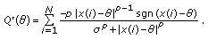 (B1)
(B1)For
 ,
,  . Then
  , which implies that
  is strictly decreasing in that interval. Similarly for
  ,
,  and
and  , showing that the function is strictly increasing in that interval.
 -
(2)
From
 we see that
  if
if  , then all local extrema of
  lie in the interval
  .
. -
(3)
Let
 for any
  . Then the objective function
  becomes
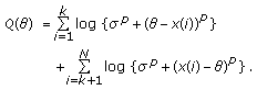 (B2)
(B2)The second derivative with respect to
 is
is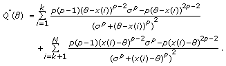 (B3)
(B3)From (B.3) it can be seen that if
 , then
  for
for  , therefore
  is concave in the intervals
  ,
,  . If all the extrema points lie in
  , the function is concave in
  , and since the function is not differentiable in the input samples
  (critical points), then the only possible local minimums of the objective function are the input samples.
 -
(4)
Consider the
 th term in
  and define
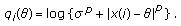 (B4)
(B4)Clearly for each
 there exists a unique minima in
  . Also, it can be easily shown that
  is convex in the interval
  , where
  , and concave outside this interval (for
  ). The proof of this statement is divided in two parts. First we consider the case when
  and show that there exist at most
  local extrema for this case. Then by induction we generalize this result for any
  .
.Let
 . If
. If  the cost function is convex in the interval
  since it is the sum of two convex functions (in that interval). Thus,
  has a unique minimizer. Now if
  , the cost function has at most one inflexion point (local maxima) between
  and at most two local minimas in the neighborhood of
  and
and  since
since  ,
,  , are concave outside the interval
  . Then, for
  we have at most
  local extrema points.
Suppose that we have
 samples. If
  , the cost function is convex in the interval
  since it is the sum of convex functions (in that interval) and it has only one global minima. Now suppose that
  , and also suppose that there are at most
  local extrema points. Let
  be a new sample in the data set, and without loss of generality assume that
  .
.If
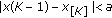 , the new sample will not add a new extrema point to the cost function, due to convexity of
  for the interval
  and the fact that
  is strictly increasing for
  . If
. If 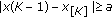 , the new sample will add at most two local extrema points (one local maxima and one local minima) in the interval
  . The local maxima is an inflexion point between
  , and the local minima is in the neighborhood of
  . Therefore, the total number of extrema points for
  is at most
  , which is the claim of the statement. This concludes the proof.
 yields
 ,
,  . Then
  , which implies that
  is strictly decreasing in that interval. Similarly for
  ,
,  and
and  , showing that the function is strictly increasing in that interval.
 we see that
  if
if  , then all local extrema of
  lie in the interval
  .
. for any
  . Then the objective function
  becomes
 is
is
 , then
  for
for  , therefore
  is concave in the intervals
  ,
,  . If all the extrema points lie in
  , the function is concave in
  , and since the function is not differentiable in the input samples
  (critical points), then the only possible local minimums of the objective function are the input samples.
 th term in
  and define
 there exists a unique minima in
  . Also, it can be easily shown that
  is convex in the interval
  , where
  , and concave outside this interval (for
  ). The proof of this statement is divided in two parts. First we consider the case when
  and show that there exist at most
  local extrema for this case. Then by induction we generalize this result for any
  .
. . If
. If  the cost function is convex in the interval
  since it is the sum of two convex functions (in that interval). Thus,
  has a unique minimizer. Now if
  , the cost function has at most one inflexion point (local maxima) between
  and at most two local minimas in the neighborhood of
  and
and  since
since  ,
,  , are concave outside the interval
  . Then, for
  we have at most
  local extrema points.
 samples. If
  , the cost function is convex in the interval
  since it is the sum of convex functions (in that interval) and it has only one global minima. Now suppose that
  , and also suppose that there are at most
  local extrema points. Let
  be a new sample in the data set, and without loss of generality assume that
  .
. , the new sample will not add a new extrema point to the cost function, due to convexity of
  for the interval
  and the fact that
  is strictly increasing for
  . If
. If  , the new sample will add at most two local extrema points (one local maxima and one local minima) in the interval
  . The local maxima is an inflexion point between
  , and the local minima is in the neighborhood of
  . Therefore, the total number of extrema points for
  is at most
  , which is the claim of the statement. This concludes the proof.
C. Proof of Property 1
Using the properties of the  function, the M-GC estimator can be expressed as

Let  . Since multiplying by a constant does not affect the result of the
  operator, we can rewrite (C.1) as

Using the fact that  and taking the limit as
  yield
yield

where the last step follows since

D. Proof of Property 2
The M-GC estimator can be expressed as

Define

Since the  function is monotone nondecreasing, the M-GC estimator can be reformulated as

It can be checked that when  is very small

where  is the number of times the value
  is repeated in the sample set and
  denotes the asymptotic order as
  . In the limit the exponent
  must be minimized for
  to be minimum. Therefore,
  will be one of the most repeated values in the input set. Define
  , then for
  , expanding the product in (D.2) gives

Since the first term in (D.5) is  , the second term is negligible for small
  . Then, in the limit,
  can be computed as

References
Kuruoglu EE: Signal processing with heavy-tailed distributions. Signal Processing 2002, 82(12):1805-1806. 10.1016/S0165-1684(02)00312-2
Barner KE, Arce GR: Nonlinear Signal and Image Processing: Theory, Methods and Applications. CRC Press, Boca Raton, Fla, USA; 2003.
Arce GR: Nonlinear Signal Processing: A Statistical Approach. John Wiley & Sons, New York, NY, USA; 2005.
Huber P: Robust Statistics. John Wiley & Sons, New York, NY, USA; 1981.
Kassam SA, Poor HV: Robust techniques for signal processing: a survey. Proceedings of the IEEE 1985, 73(3):433-481.
Astola J, Neuvo Y: Optimal median type filters for exponential noise distributions. Signal Processing 1989, 17(2):95-104. 10.1016/0165-1684(89)90013-3
Yin L, Yang R, Gabbouj M, Neuvo Y: Weighted median filters: a tutorial. IEEE Transactions on Circuits and Systems II 1996, 43(3):157-192. 10.1109/82.486465
Arce GR: A general weighted median filter structure admitting negative weights. IEEE Transactions on Signal Processing 1998, 46(12):3195-3205. 10.1109/78.735296
Shao M, Nikias CL: Signal processing with fractional lower order moments: stable processes and their applications. Proceedings of the IEEE 1993, 81(7):986-1010. 10.1109/5.231338
Barner KE, Aysal TC: Polynomial weighted median filtering. IEEE Transactions on Signal Processing 2006, 54(2):636-650.
Aysal TC, Barner KE: Hybrid polynomial filters for Gaussian and non-Gaussian noise environments. IEEE Transactions on Signal Processing 2006, 54(12):4644-4661.
Gonzales JG: Robust techniques for wireless communications in nongaussian environments, Ph.D. dissertation. ECE Department, University of Delaware; 1997.
Aysal TC, Barner KE: Meridian filtering for robust signal processing. IEEE Transactions on Signal Processing 2007, 55(8):3949-3962.
Zolotarev V: One-Dimensional Stable Distributions. American Mathematical Society, Providence, RI, USA; 1986.
Nolan JP: Stable Distributions: Models for Heavy Tailed Data. Birkhuser, Boston, Mass, USA; 2005.
Brcich RF, Iskander DR, Zoubir AM: The stability test for symmetric alpha-stable distributions. IEEE Transactions on Signal Processing 2005, 53(3):977-986.
Gonzalez JG, Arce GR: Optimality of the myriad filter in practical impulsive-noise environments. IEEE Transactions on Signal Processing 2001, 49(2):438-441. 10.1109/78.902126
Gonzalez JG, Arce GR: Statistically-efficient filtering in impulsive environments: weighted myriad filters. Eurasip Journal on Applied Signal Processing 2002, 2002(1):4-20. 10.1155/S1110865702000483
Aysal TC, Barner KE: Myriad-type polynomial filtering. IEEE Transactions on Signal Processing 2007, 55(2):747-753.
Rider PR: Generalized cauchy distributions. Annals of the Institute of Statistical Mathematics 1957, 9(1):215-223. 10.1007/BF02892507
Miller J, Thomas J: Detectors for discrete- time signals in non- Gaussian noise. IEEE Transactions on Information Theory 1972, 18(2):241-250. 10.1109/TIT.1972.1054787
Aysal TC: Filtering and estimation theory: first-order, polynomial and decentralized signal processing, Ph.D. dissertation. ECE Department, University of Delaware; 2007.
Middleton D: Statistical-physical models of electromagnetic interference. IEEE Transactions on Electromagnetic Compatibility 1977, 19(3):106-127.
Hall HM: A new model for impulsive phenomena: application to atmospheric-noise communication channels. Standford Electronics Laboratories, Standford University, Standford, Calif, USA; 1966.
Hampel F, Ronchetti E, Rousseeuw P, Stahel W: Robust Statistics: The Approach Based on Influence Functions. Wiley, New York, NY, USA; 1986.
Carrillo RE, Aysal TC, Barner KE: Generalized Cauchy distribution based robust estimation. Proceedings of IEEE International Conference on Acoustics, Speech and Signal Processing (ICASSP '08), April 2008 3389-3392.
Besag J: On the statiscal analysis of dirty pictures. Journal of the Royal Statistical Society. Series B 1986, 48(3):259-302.
McLachlan G, Krishman T: The EM Algorithm and Extensions. John Wiley & Sons, New York, NY, USA; 1997.
Hardy GH, Littlewood JE, Pólya G: Inequalities, Cambridge Mathematical Library. Cambridge University Press, Cambridge, Mass, USA; 1988.
Zimmermann M, Dostert K: Analysis and modeling of impulsive noise in broad-band powerline communications. IEEE Transactions on Electromagnetic Compatibility 2002, 44(1):249-258. 10.1109/15.990732
Ma YH, So PL, Gunawan E: Performance analysis of OFDM systems for broadband power line communications under impulsive noise and multipath effects. IEEE Transactions on Power Delivery 2005, 20(2):674-682. 10.1109/TPWRD.2005.844320
Aysal TC, Barner KE: Constrained decentralized estimation over noisy channels for sensor networks. IEEE Transactions on Signal Processing 2008, 56(4):1398-1410.
Aysal TC, Barner KE: Blind decentralized estimation for bandwidth constrained wireless sensor networks. IEEE Transactions on Wireless Communications 2008, 7(5):1466-1471.
Candès EJ, Wakin MB: An introduction to compressive sampling: a sensing/sampling paradigm that goes against the common knowledge in data acquisition. IEEE Signal Processing Magazine 2008, 25(2):21-30.
Donoho DL, Elad M, Temlyakov VN: Stable recovery of sparse overcomplete representations in the presence of noise. IEEE Transactions on Information Theory 2006, 52(1):6-18.
Haupt J, Nowak R: Signal reconstruction from noisy random projections. IEEE Transactions on Information Theory 2006, 52(9):4036-4048.
Candès EJ, Romberg JK, Tao T: Stable signal recovery from incomplete and inaccurate measurements. Communications on Pure and Applied Mathematics 2006, 59(8):1207-1223. 10.1002/cpa.20124
Tropp JA, Gilbert AC: Signal recovery from random measurements via orthogonal matching pursuit. IEEE Transactions on Information Theory 2007, 53(12):4655-4666.
Needell D, Tropp JA: CoSaMP: iterative signal recovery from incomplete and inaccurate samples. Applied and Computational Harmonic Analysis 2009, 26(3):301-321. 10.1016/j.acha.2008.07.002
Candès EJ, Randall PA: Highly robust error correction by convex programming. IEEE Transactions on Information Theory 2008, 54(7):2829-2840.
Popilka B, Setzer S, Steidl G: Signal recovery from incomplete measurements in the presence of outliers. Inverse Problems and Imaging 2007, 1(4):661-672.
Carrillo RE, Barner KE, Aysal TC: Robust sampling and reconstruction methods for sparse signals in the presence of impulsive noise. IEEE Journal on Selected Topics in Signal Processing 2010, 4(2):392-408.
Dave RN: Characterization and detection of noise in clustering. Pattern Recognition Letters 1991, 12(11):657-664. 10.1016/0167-8655(91)90002-4
Dave RN, Krishnapuram R: Robust clustering methods: a unified view. IEEE Transactions on Fuzzy Systems 1997, 5(2):270-293. 10.1109/91.580801
Yang M-S, Wu K-L: A similarity-based robust clustering method. IEEE Transactions on Pattern Analysis and Machine Intelligence 2004, 26(4):434-448. 10.1109/TPAMI.2004.1265860
Papoulis A: Probability, Random Variables, and Stochastic Processes. McGraw-Hill, New York, NY, USA; 1984.
Acknowledgment
This paper was supported in part by NSF under Grant no. 0728904.
Author information
Authors and Affiliations
Corresponding author
Rights and permissions
Open Access This article is distributed under the terms of the Creative Commons Attribution 2.0 International License (https://creativecommons.org/licenses/by/2.0), which permits unrestricted use, distribution, and reproduction in any medium, provided the original work is properly cited.
About this article
Cite this article
Carrillo, R.E., Aysal, T.C. & Barner, K.E. A Generalized Cauchy Distribution Framework for Problems Requiring Robust Behavior. EURASIP J. Adv. Signal Process. 2010, 312989 (2010). https://doi.org/10.1155/2010/312989
Received:
Revised:
Accepted:
Published:
DOI: https://doi.org/10.1155/2010/312989