- Research
- Open access
- Published:
An efficient voice activity detection algorithm by combining statistical model and energy detection
EURASIP Journal on Advances in Signal Processing volume 2011, Article number: 18 (2011)
Abstract
In this article, we present a new voice activity detection (VAD) algorithm that is based on statistical models and empirical rule-based energy detection algorithm. Specifically, it needs two steps to separate speech segments from background noise. For the first step, the VAD detects possible speech endpoints efficiently using the empirical rule-based energy detection algorithm. However, the possible endpoints are not accurate enough when the signal-to-noise ratio is low. Therefore, for the second step, we propose a new gaussian mixture model-based multiple-observation log likelihood ratio algorithm to align the endpoints to their optimal positions. Several experiments are conducted to evaluate the proposed VAD on both accuracy and efficiency. The results show that it could achieve better performance than the six referenced VADs in various noise scenarios.
1 Introduction
Voice activity detector (VAD) segregates speeches from background noise. It finds diverse applications in many modern speech communication systems, such as speech recognition, speech coding, noisy speech enhancement, mobile telephony, and very small aperture terminals. During the past few decades, researchers have tried many approaches to improve the VAD performance. Traditional approaches include energy in time domain [1, 2], pitch detection [3], and zero-crossing rate [2, 4]. Recently, several spectral energy-based new features were proposed, including energy-entropy feature [5], spacial signal correlation [6], cepstral feature [7], higher-order statistics [8, 9], teager energy [10], spectral divergence [11], etc. Multi-band technique, which utilized the band differences between the speech and the noise, was also employed to construct the features [12, 13].
Meanwhile, statistical models have attracted much attention. Most of them were focused on finding a suitable model to simulate the empirical distribution of the speech. Sohn [14] assumed that the speech and noise signals in discrete Fourier transform (DFT) domain were independent gaussian distribution. Gazor [15] further used Laplace distribution to model the speech signals. Chang [16] analyzed the Gaussian, Laplace, and Gamma distributions in DFT domain and integrated them with goodness-of-fit test. Tahmasbi [17] supposed speech process, which was transformed by GARCH filter, having a variance gamma distribution. Ramirez [18] proposed the multiple-observation likelihood ratio test instead of the single frame LRT [14], which improved the VAD performance greatly. More recently, many machine learning-based statistical methods were proposed and have shown promising performances. They include uniform most powerful test [19], discriminative (weight) training [20, 21], support vector machine (SVM) [22–24], etc.
On the other hand, because the speech signals were difficult to be captured perfectly by feature analysis, many empirical rules were constructed to compensate the drawbacks of the VADs. Ramirez [18] proposed the contextual multiple global hypothesis to control the false alarm rate (FAR), where the empirical minimum speech length was used as the premise of his global hypothesis. ETSI frame dropping (FD) VAD [25] was somewhat an assembly of rules that were based on the continuity of speech. Besides, to our knowledge, one widely used empirical technique was the "hangover" scheme. Davis [26] designed a state machine-based hangover scheme to improve the SDR. Sohn [14] used the hidden Markov model (HMM) to cover the trivial speeches, and Kuroiwa [27] designed a grammatical system to enhance the robustness of the VAD.
The statistical models could detect the voice activity exactly, but they are not efficient in practice. On the other hand, the empirical rules could not only distinguish the apparent noise from speech but also cover trivial speeches; however, they are not accurate enough in detecting the endpoints. In this article, we propose a new VAD algorithm by combining the empirical rule-based energy detection algorithm and the statistical models together. The rest of the article is organized as follows. In Section 2, we will present the empirical rule-based energy detection sub-algorithm and the Gaussian mixture model (GMM)-based multiple-observation log likelihood ratio (MO-LLR) sub-algorithm in detail, and then we will present how the two independent sub-algorithms are combined. In Section 3, several experiments are conducted. The results show that the proposed algorithm could achieve better performances than the six existing algorithms in various noise scenarios at different signal-to-noise ratio (SNR) levels. In Section 4, we conclude this article and summarize our findings.
2 The proposed efficient VAD algorithm
2.1 The proposed VAD algorithm in brief
In [28], Li summarized some general requirements for a practical VAD. In this article, we conclude them as follows and take them as the objective for the proposed algorithm.
-
1)
Invariant outputs at various background energy levels, with maximum improvements of speech detection.
-
2)
Accurate location of detected endpoints.
-
3)
Short time delay or look-ahead.
If we use only one algorithm, then it is hard to satisfy the second and third items simultaneously. If the average SNR level of current speech signals is above zero, then the short-term SNRs around the speech endpoints are usually much lower than those between the endpoints. Hence, we could use different detection schemes for different part of one speech segment.
The proposed algorithm has two steps to separate speech segments from background noise. For the first step, we use the double threshold energy detection algorithm [2] to detect the possible endpoints of the speech segments efficiently. However, the detected endpoints are rough. Therefore, for the second step, we use the GMM based MO-LLR algorithm to search around the possible endpoints for the accurate ones.
By doing so, only signals around the endpoints need the computationally expensive algorithm. Therefore, a lot of detecting time could be saved.
2.2 Empirical rules-based energy detection
The efficient energy detection algorithm is not only to detect the apparent speeches but also to find the approximate positions of the endpoints. However, the algorithm is not robust enough when the SNR is low. To enhance its robustness, we integrate it with a group of rules and present it as follows:
Part1 As for the beginning-point (BP) detection, the silence energy and the low\high energy thresh-olds of the n th observation o n are defined as


where E j is the short-term energy of the j th observation; and the α, β are the user-defined threshold factors.
Given a signal segment {o
n
, o
n
+1, ..., o
n
+ NB-1} with a length of N
B
observations, if there are  consecutive observations in the segment whose energy is higher than Thlow, and if the ratio
  is higher than an empirical threshold
  , then the first observation
  energy is higher than Thlow, should be remembered.
Then, we detect the given segment from  ; if there is another
  consecutive observation whose energy is higher than Thhigh, and if the ratio
  is higher than another empirical threshold
  , then one possible BP is detected as ô
B
.
, then one possible BP is detected as ô
B
.
Part2 As for the ending-point (EP) detection, suppose that the energy of current observation ô
E
is lower than Thlow; we analyze its subsequent signal segment with N
E
observations. If there are  observations with energy higher than Thhigh in the segment, and if the ratio
  is lower than an empirical threshold φEP, then one possible EP is detected as the current observation ô
E
.
is lower than an empirical threshold φEP, then one possible EP is detected as the current observation ô
E
.
2.3 GMM-based MO-LLR algorithm
Although the energy-based algorithm is efficient to detect speech signals roughly, the endpoints detected by it are not sufficiently accurate. Therefore, some computationally expensive algorithm is needed to detect the endpoints accurately. Here, a new algorithm called the GMM-based MO-LLR algorithm is proposed.
Given the current observation o n , a window {o n-l , ..., o n -1, o n , o n +1, ..., o n + m } is defined over o n . Acoustic features {x n - l , ..., x n + m }a are extracted from the window. Two K-mixture GMMs are employed to model the speech and noise distributions, respectively:


where i = n - l, ..., n + m, H1 (H0) denotes the hypothesis of the speech (noise), and {π k , μ k , Σ k } are the parameters of the k th mixture.
Base on the above definition, the log likelihood ratio (LLR) s i of the observation o i can be calculated as

and the hard decision on s i is obtained by

where ε is employed to tune the operating point of a single observation. In practice, ε is initialized as  , where the first term denotes the current SNR level, and Δ is a user-defined constant. The constant "15" can be set to other value too.
Until now, we can obtain a new feature vector I n = {s n - l , ..., s n + m }T (or I n = {c n - l , ..., c n + m }T) from the soft (or hard) decision. Many classifiers based on the new feature can be designed, such as the most simplest one calculating the average value of the feature [29], the global hypothesis on the multiple observation [18], the long-term amplitude envelope method [22], and the discriminative (weight) training method of the feature [20, 21]. For simplicity, we just calculate the average value of the feature:

and classify the current observation o n by

where η is employed to tune the operating point of the MO-LLR algorithm.
Figure 1 gives an example of the detection process of the MO-LLR sub-algorithm with l = m - 1. From the figure, we could know that when the window length becomes large, the proposed algorithm has a good ability of controlling the randomness of the speech signals but a relatively weak ability of detecting very short pauses between speeches. Therefore, setting the window to a proper length is important to balance the performance between the speech detection accuracy and the FAR.

MO-LLR scores (SNR = 15 dB). The vertical solid lines are the endpoints of the utterance. The transverse dotted lines are the decision thresholds. (a) Single observation LLR scores. (b) Soft MO-LLR scores with a window length of 10. (c) Soft MO-LLR scores with a window length of 30. (d) Hard-decision output of the MO-LLR algorithm with a window length of 30. Threshold for the hard-decision is 1.5.
In our study, the hard decision method (6) is adopted, and two thresholds, η begin and η end , are used for the BP and EP detections, respectively, instead of a single η in (8).
2.4 Combination of the energy detection algorithm and the MO-LLR algorithm
The main consideration of the combination is to detect the noise\speech signals that can be easily differentiated by the energy detection algorithm at first, leaving the signals around the endpoints to the MO-LLR sub-algorithm.
Figure 2 gives a direct explanation of the combination method. From the figure, it is clear that the MO-LLR sub-algorithm is only used around the possible endpoints that are detected by the energy detection algorithm. Hence, a lot of computation can be saved.

Schematic diagram of the proposed combination algorithm.
We summarize the proposed algorithm in Algorithm 1 with its state transition graph drawn in Figure 3. Note that for the MO-LLR sub-algorithm, because an observation might appear not only in the current window but also in the next window when the MO-LLR window shifts, its output value from Equation 5 or 6 might be used several times. Therefore, the MO-LLR output of any observation should be remembered for a few seconds to prevent repeating calculating the LLR score in (5).

State transition diagram of the proposed algorithm. The number "1" denotes that the speech observation is detected; "0" denotes that the noise observation is detected. "E" is short for the energy detection sub-algorithm; "G" is short for the GMM based MO-LLR sub-algorithm.
2.5 Considerations on model training
2.5.1 Matching training for MO-LLR sub-algorithm
The observations between the endpoints have higher energy than those around the endpoints, and they have different spacial distributions with those around the endpoints too.
In our proposed algorithm, the input data of the MO-LLR sub-algorithm is just the observations around the endpoints. If we use all data for training, then it is obvious that the mismatching between the distribution of the speeches around the endpoints and the distribution of the speeches on the entire dataset will lower the classification accuracy of the data around the endpoints. Therefore, we only use the observations around the endpoints for GMM training. The expectation-maximum (EM) algorithm is used for GMM training.
2.5.2 Selections of the training dataset
In practice, to find the training dataset that matches the test environment perfectly is difficult. Hence, we need a VAD algorithm that is not sensitive to the selections of the training dataset.
To find how much the mismatching between the training and the test sets will affect the performance, we define two kinds of models as follows:
-
Noise-dependent model (NDM). This kind of model is trained in a given noise environment, and is only tested in the same environment.
-
Noise-independent model (NIM). This kind of model is trained from a training set that is a collection of speeches in various noise environments, and is tested in arbitrary noise scenarios.
The performance of the NDM is thought to be better than NIM. However, we will show in our experiments that the NIM could achieve similar performance with the NDM, which proves the robustness of the proposed algorithm.
In conclusion, constructing a training dataset that consists of various noise environments is sufficient for the GMM training in practice.
2.6 Extensions and limitations of the proposed algorithm
The proposed combination method is easily extended to other features and classifiers. Many efficient algorithms can replace the energy detection algorithm, and besides MO-LLR algorithm, many accurate algorithms can be used to detect the precise positions of the endpoints too. If designed properly, then we can combine the two complementary sub-algorithms in our proposed method so as to inherit both of their advantages.
To better understand the idea, we construct a new combination algorithm using two other sub-algorithms, where the sub-algorithms were proposed by other researchers.
-
Efficient sub-algorithm. In [28], a new feature is defined as
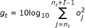 (9)
(9)

where o j is the j th sample in time domain, I is the user-defined window length, and n t is the index of the first sample in the window. Instead of using Li's system [28] directly, we can just use the feature to replace ours in the energy detection part.
-
Accurate sub-algorithm. In [22], Ramirez proposed a new feature vector for SVM-based VAD. It was inspired by [28]. We present it briefly as follows. After DFT analysis of an observation, an N-dimensional vector
 is obtained. In each dimension of the feature, the long-term spectral envelope can be calculated as
  , where l is the user-defined window length. Then, we transform the feature vector to another K-band spectral representation [22]
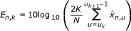 (10)
(10)
 is obtained. In each dimension of the feature, the long-term spectral envelope can be calculated as
  , where l is the user-defined window length. Then, we transform the feature vector to another K-band spectral representation [
where u k =⌊N/2·k/K⌋ and k = 0, 1, ..., K - 1. Eventually, the element of the feature vector z n for SVM is defined as z n, k = E n, k - V n, k , where the spectral representation of the noise V n, k is estimated in the same way as E n, k during the initialization period and the silence period. In [22], Ramirez has shown that the SVM-based VAD could achieve higher classification accuracy than Li's [28].
However, the computational complexity has not been considered. The nonlinear kernel SVM [30]-based VAD has been proved to be superior to the linear kernel SVM-based VAD [23, 24]. However, if we use the nonlinear kernel SVM, then the following calculation is traditionally needed to classify a single observation o n :

where  are the non-negative lagrange variables,
  is the nonlinear kernel operator, T denotes the total observation number of the training set, and
  is the training dataset. Therefore, the time complexity for classifying a single observation is even as high as
  which is unbearable in practice.
-
Combination of the two sub-algorithms. The two algorithms can be combined efficiently by modifying the sample o j in time domain (in Equation 9) to the observations in spectral domain.
Obviously, even after the combination, the time complexity of the above algorithm is much higher than our proposed method. Therefore, we never tried to realize it.
Although the proposed combination method is easily extended, it has one limitation as well. It is weak in detecting very short pauses between speeches. This is because we mainly try to optimize the detecting efficiency instead of pursuing the highest accuracy. If the applications need to detect the short pauses accurately, then we might overcome the drawback by adding some new rules or some complementary algorithms to the energy detection part.
3 Experimental analysis
In this section, we will compare the performances of the proposed algorithm with the other referenced VADs in general at first. Then, we will analyze its efficiency in respect of the mixture number of the GMM and the combination scheme. At last, we will prove that the proposed algorithm can achieve robust performance in mismatching situation between the training and test sets.
3.1 Experimental setup
The TIMIT [31] speech corpus is used as the dataset. It contains utterances from eight different dialect regions in the USA. It consists of a training set of 326 male and 136 female speakers, and a testing set of 112 male and 56 female speakers. Each speakers utters 10 sentences, so that there are 4,620 utterances in the training set and 1,680 utterances in the test set totally. All the recorded speech signals are sampled at fs = 16 kHz.
These TIMIT sets, after resampling from 16 to 8 kHz, are distorted artificially by the NOISEX corpus [32]. To simulate the real-world noise environment, the original TIMIT and NOISEX corpora are filtered by intermediate reference system [33] to simulate the phone handset, and then the SNR estimation algorithm based on active speech level [34] is employed to add four different noise types (babble, factory, vehicle, and white noise) at five SNR levels in a range of [5, 10,..., 25 dB]. Eventually, we get 20 pairs of noise-distorted training and test corpora. As done in a previous study [35], the TIMIT word transcription is used for VAD evaluation, and the inactive speech regions, which are smaller than 200 ms, are set to speech. The percentage of the speech process is 87.78%, which is much higher than the average level of the true application environments. To make the corpora more suitable for VAD evaluation, every utterance is artificially extended at the head and the tail, respectively, with some noise. The percentage of the speech is afterwards reduced to 62.83%, and the renewed corpora can reflect the differences of the VADs apparently.
To examine the effectiveness of the proposed VAD algorithm, we compare it with the following existing VAD methods.
-
G.729B VAD [4]. It is a standard method applied for improving the bandwidth efficiency of the speech communication system. Several traditional features and methods are arranged in parallel.
-
VAD from ETSI AFE ES 202 050 [25]. It is the front-end model of an European standard speech recognition system. It consists of two VADs. The first one, called "AFE Wiener filtering (WF) VAD," is based on the spectral SNR estimation algorithm. The second one, called "AFE FD VAD", is a set of empirical rules. Its main purpose is to integrate the fragmental output from AFE WF VAD into speech segments.
-
Sohn VAD [14]. It is a statistical model-based VAD. It uses the minimum-mean square error estimation algorithm [36] to estimate the spectral SNR, and the gaussian model to model the distributions of the speech and noise.
-
Ramirez VAD [18]. It combines the multiple-observation technique [11, 29] and the statistical VAD at first, and then, it proposes the global hypothesis to control the FAR.
-
Tahmasbi VAD [17]. It assumes that the speeches, after being filtered by GARCH model, have a variance gamma distribution. We train the GARCH model in matching environment between the training and test sets.
3.2 Parameter settings
A single observation (frame) length is 25 ms long with an overlap of 10 ms.
For the rule-based energy detection algorithm, N
B
in the BP detection is set to 20 with  and
and  . The N
E
in EP detection is set to 35 with φEP = 1/7.
. The N
E
in EP detection is set to 35 with φEP = 1/7.
For the MO-LLR algorithm, the 39-dimensional feature contains 13-dimensional static MFCC features (with energy and without C0), their delta and delta-delta features. The window length is set to 30 with l setting to 14. The constant Δ referred in (6) is set to 1.5.
For the combination of the two sub-algorithms (Algorithm 1), the scanning range δ is set to 50. The minimum practical speech length is set to 35.
Other parameters related to SNR are show in Table 1. These values are the optimal ones in different SNR levels. We get them from the training set of the noisy TIMIT corpora.
In respect of matching training for MO-LLR sub-algorithm, 50 neighboring observations of every endpoint are extracted from the training set for GMM training.
In respect of the selections of the training dataset, two kinds of models should be trained for performance comparison.
For the NIM training, we randomly extract 231 utterances from every noise-distorted training corpus to form a noise-independent training corpus, and then we train a serial GMM pairs with [1, 2, 3, 5, 15, 35, and 50] mixtures correspondingly. Note that the new noise-independent corpus contains 4,620 utterances totally, which is the same size as each noise-distorted training set.
For the NDM training, we train 20 pairs of 50-mixture NDMs from 20 noisy corpora.
3.3 Results
3.3.1 Performance comparison with referenced VADs
Two measures are used for evaluation. One measure is the speech detection rate (SDR) and the FAR [37]. In order to evaluate the performance in a single variable, another measure is the harmonic mean F-score [35] between the precision rate of the detected speeches (PR) and the SDR

The higher the F-score is the better the VAD performs.
Table 2 lists the performance comparisons of the proposed algorithm (with 5-mixture NIM) with other existing VADs. From the table, the G.729B, the AFE WF, and AFE FD VAD, which are open sources, have relatively comparable performances with the Sohn, Ramirez, and Tahmasbi VAD. This conclusion is identical with other studies, e.g., [14, 18, 35]. Also, the performances of the proposed algorithm are better than other referenced VADs. Figure 4 shows the F-score comparisons of the VADs. From the figure, we can see that the proposed algorithm yields higher F-score curves than other VADs.

F -score comparisons in different noise scenarios.
Table 3b lists the average CPU time of the proposed algorithm (with 5-mixtures NIM) and the referenced statistical model-based VADs over all 20 noisy corpora. From the table, it is clear that the proposed algorithm is faster than the three statistical VADs. The reason for the Sohn VAD being slower than Ramirez VAD is that the HMM-based "hangover" scheme in Sohn VAD is computationally expensive.
3.3.2 How does the mixture number of the GMM affect the performance?
If the mixture number of the GMM increases, then it is preferred that the performance of the VAD will be better. However, the computational complexity increases with the mixture number too. Therefore, it is important to find how the mixture number of the GMM will affect the performance and how many mixtures are needed to compromise the detecting time and the accuracy.
The first row of Table 4 lists the average CPU time of the proposed methods with different mixture numbers over all the 20 noisy corpora. From the row, a linear relationship between the mixture number and the CPU time is observed.
Table 5 shows the average accuracy of the proposed methods with different mixture numbers over all the noisy corpora. From the table, we can see that the mixture number has little effect on the performance when the number is larger than 5.
In conclusion, setting the mixture number to 5 is enough to guarantee the detecting accuracy.
3.3.3 How much time could be saved by using the combination algorithm instead of using MO-LLR only?
In order to show the advantage of the combination, we compare the proposed algorithm with the MO-LLR algorithm.
Table 4 gives the CPU time comparison between the proposed algorithm and the MO-LLR algorithm. From the table, we can conclude that the proposed algorithm is several times faster than the MO-LLR algorithm.
3.3.4 How does the mismatching between the training and the test sets affect the performance?
The histograms of the differences between the manually labeled endpoints and the detected ones [28] is used as the measure. The main reason for using this measure is that the MO-LLR sub-algorithm is only used in the area around the endpoints but not over the entire corpora.
Figure 5 gives an example of the histograms. It is clear that the BP is much easier detected than the EP.

The accumulating results (histograms) of the differences between the manually labeled endpoints and the detected ones in different noise scenarios. Each column of the histogram is in a width of five observations. If the detected endpoint is in the positive axis of the histogram, it means that the noises between the detected one and the labeled one are wrongly detected as speech, vise versa.
However, since there are too many histograms to show in this article, we substitute the histograms by their means and standard deviations. The closer to zero the means and variances are, the better the GMMs perform.
Table 6 lists the average results of the means of the histograms over all the noisy corpora. It is shown that the performance of the NDM is not much better than the NIM, especially when they have the same mixture number, which proves the robustness of the proposed algorithm. From the NIM column only, we could also conclude that the performances change slightly from 5 to 50 mixtures.
To summarize, in order to achieve robust performance, we just need to train 5-mixture GMMs from a dataset that consists of various noisy environments instead of training new GMMs for each new test environment. Eventually, the trouble on training new models can be avoided.
4 Conclusions
In this article, we present an efficient VAD algorithm by combining two sub-algorithms. The first sub-algorithm is the efficient rule-based energy detection algorithm, where the rules can enhance the robustness of the energy detection algorithm. The second sub-algorithm is the GMM-based MO-LLR algorithm. Although the MO-LLR is computationally expensive, it can classify the speech and noise accurately. The two sub-algorithms are combined by first using the energy detection algorithm to detect the speeches that are easily differentiated, leaving the speeches around the endpoints to the MO-LLR sub-algorithm. The experimental results show that the proposed algorithm could achieve better performances than the six commonly used VADs. It has also been demonstrated that the proposed VAD is more efficient and robust in different noisy environments.
Endnotes
aHere, we use the MFCC, its delta and delta-delta features as the feature, which has a total dimension of 39. But the proposed method is not limited to the feature. bBecause the G.729B VAD and ETSI AFE VAD are implemented in C code but the other four is implemented in MATLAB code, it's meaningless to compare the proposed algorithm with the G.729B VAD and ETSI AFE VAD directly.
Algorithm 1: Combining energy detection & MO-LLR
1: initialization start from silence.
BP detection:
2: if a possible BP ô B is detected by Part1 of the energy detection
3: if ô B is confirmed to be speech by MO-LLR
4: search in a range of (ô B -δ, ô B +δ) for the accurate
o B BP by MO-LLR. o B is defined as the change point from noise to speech.
5: goto the ending-point detection (Step 12)
6: else
7: move to next observation, goto Step 2
8: end
9: else
10: move to next observation, goto Step 2
11: end
ending-point (EP) detection:
12: if a possible EP ô E is detected by Part2 of the energy detection
13: if ô E is confirmed to be noise by MO-LLR
14: search in a range of (ô E -δ, ô E +δ) for the accurate EP
o E by MO-LLR. o E is defined as the change point
from speech to noise.
15: if the length from o B to o E is too small to be practical
16: delete the detected speech endpoints o B and o E
17: end
18: goto the BP detection (Step 2)
19: else
20: move to next observation, goto Step 12.
21: end
22: else
23: move to next observation, goto Step 12.
24: end
Abbreviations
- DFT:
-
discrete Fourier transform
- EM:
-
expectation-maximum
- FAR:
-
false alarm rate
- FD:
-
frame dropping
- GMM:
-
Gaussian mixture model
- HMM:
-
hidden Markov model
- LLR:
-
log likelihood ratio
- MO-LLR:
-
multiple-observation log likelihood ratio
- NDM:
-
noise-dependent model
- NIM:
-
noise-independent model
- SDR:
-
speech detection rate
- SNR:
-
signal-to-noise ratio
- SVM:
-
support vector machine
- VAD:
-
voice activity detection.
References
Wilpon JG, Rabiner LR, Martin T: "An improved word detection algorithm for telephone-quality speech incorporating both syntactic and semantic constraints". AT&T Bell Labs Tech J 1984, 63: 353-364.
Rabiner LR, Sambur MR: "An algorithm for determining the endpoints of isolated utterances". Bell Sys Tech J 1975,54(2):297-315.
Chengalvarayan R: "Robust energy normalization using speech/nonspeech discriminator for German connected digit recognition". 6th Euro Conf Speech Commun, Tech, ISCA 1999.
Benyassine A, Shlomot E, Su HY, Massaloux D, Lamblin C, Petit JP: "ITU-T Recommendation G. 729 Annex B: a silence compression scheme for use with G. 729 optimized for V. 70 digital simultaneous voice and data applications". IEEE Commun Mag 1997,35(9):64-73. 10.1109/35.620527
Huang L, Yang C: "A novel approach to robust speech endpoint detection in carenvironments". Proc Int Conf Acoust, Speech and Signal Process 2000., 3:
Le Bouquin-Jeannès R, Faucon G: "Study of a voice activity detector and its influence on a noise reduction system". Speech Commun 1995,16(3):245-254. 10.1016/0167-6393(94)00056-G
Shen J, Hung J, Lee L: "Robust entropy-based endpoint detection for speech recognition in noisy environments". 5th Int Conf Spoken Lang Process 1998.
Nemer E, Goubran R, Mahmoud S: "Robust voice activity detection using higher-order statistics in the LPC residual domain". IEEE Trans Acoust, Speech, Signal Process 2001,9(3):217-231.
Li K, Swamy M, Ahmad M: "An improved voice activity detection using higher order statistics". IEEE Trans Acoust, Speech, Signal Process 2005,13(5 Part 2):965-974.
Ying G, Jamieson L, Mitchell C: "Endpoint detection of isolated utterances based on a modified Teager energy measurement". Int Conf Acoust, Speech, Signal Process 1993., 2:
Ramírez J, Segura J, Benitez C, De La Torre A, Rubio A: "Efficient voice activity detection algorithms using long-term speech information". Speech Communi 2004,42(3-4):271-287. 10.1016/j.specom.2003.10.002
Evangelopoulos G, Maragos P: "Multiband modulation energy tracking for noisy speech detection". IEEE Trans Audio, Speech Lang Process 2006,14(6):2024-2038.
Wu B-F, Wang K: "Robust endpoint detection algorithm based on the adaptive band-partitioning spectral entropy in adverse environments". IEEE Trans Acoust, Speech, Signal Process 2005,13(5):762-775.
Sohn J, Kim NS, Sung W: "A statistical model-based voice activity detection". IEEE Signal Process Lett 1999,6(1):1-3. 10.1109/97.736233
Gazor S, Zhang W: "A soft voice activity detector based on a Laplacian-Gaussian model". IEEE Trans Acoust, Speech, Signal Process 2003,11(5):498-505.
Chang JH, Kim NS, Mitra SK: "Voice activity detection based on multiple statistical models". IEEE Trans Signal Process 2006,54(6):1965-1976.
Tahmasbi R, Rezaei S: "A soft voice activity detection using GARCH filter and variance Gamma distribution". IEEE Trans Audio, Speech Lang Process 2007,15(4):1129-1134.
Ramírez J, Segura JC, Górriz JM, García L: "Improved voice activity detection using contextual multiple hypothesis testing for robust speech recognition". IEEE Trans Audio, Speech Lang Process 2007,15(8):2177-2189.
Kim D, Jang K, Chang J: "A new statistical voice activity detection based on ump test". IEEE Signal Process Lett 2007,14(11):891-894.
Kang S, Jo Q, Chang J: "Discriminative weight training for a statistical model based voice activity detection". IEEE Signal Process Lett 2008, 15: 170-173.
Yu T, Hansen JHL: "Discriminative training for multiple observation likelihood ratio based voice activity detection". IEEE Signal Process Lett 2010,17(11):897-900.
Ramírez J, Yélamos P, Górriz J, Segura J: "SVM-based speech endpoint detection using contextual speech features". Electron Let 2006,42(7):426-428. 10.1049/el:20064068
Jo Q, Chang J, Shin J, Kim N: "Statistical model based voice activity detection using support vector machine". IET Signal Process 2009,3(3):205-210. 10.1049/iet-spr.2008.0128
Shin JW, Chang JH, Kim NS: "Voice activity detection based on statistical models and machine learning approaches". Computer Speech & Language 2010,24(3):515-530. 10.1016/j.csl.2009.02.003
ETSI: "Speech processing, transmission and quality aspects (STQ); distributed speech recognition; advanced front-end feature extraction algorithm; compression algorithms". ETSI ES 202(050):
Davis A, Nordholm S, Togneri R: "Statistical voice activity detection using low-variance spectrum estimation and an adaptive threshold". IEEE Trans Audio, Speech Lang Process 2006,14(2):412-424.
Kuroiwa S, Naito M, Yamamoto S, Higuchi N: "Robust speech detection method for telephone speech recognition system". Speech Commun 1999, 27: 135-148. 10.1016/S0167-6393(98)00072-7
Li Q, Zheng J, Tsai A, Zhou Q: "Robust endpoint detection and energy normalization for real-time speech and speaker recognition". IEEE Trans Acoust, Speech, Signal Process 2002,10(3):146-157.
Ramírez J, Segura JC, Benítez C, Garcìa L, Rubio A: "Statistical voice activity detection using a multiple observation likelihood ratio test". IEEE Signal Process Lett 2005,12(10):689-692.
Schölkopf B, Smola AJ: Learning With Kernels. MIT Press, Cambridge, MA; 2002.
Garofolo J, Lamel L, Fisher W, Fiscus J, Pallett D, Dahlgren N: "DARPA TIMIT acoustic-phonetic continuous speech corpus CD-ROM". NTIS order number PB91-100354 1993.
The Rice University, "Noisex-92 database"[http://spib.rice.edu/spib]
ITU-T Rec P.48: Specifications for an intermediate reference system. ITU-T; 1989.
ITU-T Rec P.56: Objective measurement of active speech level. ITU-T; 1993.
Pham TV, Tang CT, Stadtschnitzer M: "Using artificial neural network for robust voice activity detection under adverse conditions". Int Conf Comput, Commun Tech, RIVF '09 2009, 1-8.
Ephraim Y, Malah D: "Speech enhancement using a minimum-mean square error short-time spectral amplitude estimator". IEEE Trans Audio, Speech Lang Proc 1984,32(6):1109-1121.
Kay S: Fundamentals of Statistical signal processing, Volume 2: Detection theory. Prentice Hall PTR; 1998.
Acknowledgements
This study was supported by The National High-Tech. R&D Program of China (863 Program) under Grant 2006AA010104.
Author information
Authors and Affiliations
Corresponding author
Additional information
Competing interests
The authors declare that they have no competing interests.
Authors’ original submitted files for images
Below are the links to the authors’ original submitted files for images.
Rights and permissions
Open Access This article is distributed under the terms of the Creative Commons Attribution 2.0 International License (https://creativecommons.org/licenses/by/2.0), which permits unrestricted use, distribution, and reproduction in any medium, provided the original work is properly cited.
About this article
Cite this article
Wu, J., Zhang, XL. An efficient voice activity detection algorithm by combining statistical model and energy detection. EURASIP J. Adv. Signal Process. 2011, 18 (2011). https://doi.org/10.1186/1687-6180-2011-18
Received:
Accepted:
Published:
DOI: https://doi.org/10.1186/1687-6180-2011-18