Dynamic artificial bee colony algorithm for multi-parameters optimization of support vector machine-based soft-margin classifier

Abstract

This article proposes a ‘dynamic’ artificial bee colony (D-ABC) algorithm for solving optimizing problems. It overcomes the poor performance of artificial bee colony (ABC) algorithm, when applied to multi-parameters optimization. A dynamic ‘activity’ factor is introduced to D-ABC algorithm to speed up convergence and improve the quality of solution. This D-ABC algorithm is employed for multi-parameters optimization of support vector machine (SVM)-based soft-margin classifier. Parameter optimization is significant to improve classification performance of SVM-based classifier. Classification accuracy is defined as the objection function, and the many parameters, including ‘kernel parameter’, ‘cost factor’, etc., form a solution vector to be optimized. Experiments demonstrate that D-ABC algorithm has better performance than traditional methods for this optimizing problem, and better parameters of SVM are obtained which lead to higher classification accuracy.

Introduction

Artificial bee colony (ABC) algorithm was first proposed by Karaboga in 2005 [1]. It has many advantages than earlier swarm intelligence algorithms, especially for constrained optimization problem.

A constrained optimization problem (1) is defined as finding solution $\overrightarrow{\text{x}}$ that minimizes an objective function $f\left(\overrightarrow{\text{x}}\right)$ subject to inequality and/or equality constraints [2]:

$$\begin{array}{l}\text{minimize}\begin{array}{cc}\hfill f\left(\overrightarrow{\text{x}}\right),\hfill & \hfill \overrightarrow{\text{x}}\hfill \end{array}=(x_1,\dots ,x_D)\in {\mathfrak{R}}^D\\ \begin{array}{c}\hfill l_i\le x_i\le u_i,\hfill \end{array}\begin{array}{c}\hfill i=1,\dots ,D\hfill \end{array}\\ \text{subject}\begin{array}{c}\hfill \text{to}:\hfill \end{array}\begin{array}{c}\hfill g_j\left(\overrightarrow{\text{x}}\right)\le 0,\hfill \end{array}\begin{array}{c}\hfill for\begin{array}{c}\hfill j=1,\dots ,q\hfill \end{array}\hfill \end{array}\\ \begin{array}{c}\hfill h_j\left(\overrightarrow{\text{x}}\right)=0,\begin{array}{c}\hfill \begin{array}{}\end{array}for\begin{array}{c}\hfill j=q+1,\dots ,m\hfill \end{array}\hfill \end{array}\hfill \end{array}\end{array}$$

(1)

when D is larger and each element of $\overrightarrow{\text{x}}$ represents a specific parameter, it is a multi-parameters optimization problem.

Simulating the foraging behavior of honey bee swarm, ABC algorithm assumes solution $\overrightarrow{\text{x}}$ as coordinate of nectar source in D-dimensional space, and defines objective function $f\left(\overrightarrow{\text{x}}\right)$ which reflects quality of the nectar source. Small value of objective function indicates better nectar source. As bee swarm continually searching better nectar source, the algorithm could find the best solution $\overrightarrow{\text{x}}$.

However, ABC algorithm is criticized owing to its poor convergence rate and local optimization problems [3–6]. Many modified methods have been proposed. As the earlier idea of many researchers, poor performance is attributed to ‘roulette wheel’ selection mechanism, which is introduced in the onlooker phase of the original ABC algorithm. Boltzmann selection mechanism was employed instead of roulette wheel selection by Haijun and Qingxian [7]. Interactive ABC, proposed by Tsai et al. [8], introduced the Newtonian law of universal gravitation, which was also for modifying the original selection mechanism. Akbari et al. [9] proposed a modified formula for different phases of ABC algorithm. Actually, according to testing by abundant experiments, these modified methods could improve the original algorithm only when D is not too large. Nevertheless, our findings provide evidence that it is the ‘randomly single element modification (RSEM) process’, which principally leads ABC algorithm to poor performance. In traditional ABC algorithm, for each memorized solution $\overrightarrow{\text{x}}$, modifying operation is on single element x _k (k∈[1,D) of $\overrightarrow{\text{x}}$ in each cycle, and solution $\overrightarrow{\text{x}}$ changes little after each modification. Moreover, element x _k is randomly selected. It is uncertain whether the modification of x _k could improve the solution $\overrightarrow{\text{x}}$, particularly when D is large. Consequently, more cycles are needed for searching best solution, and the algorithm performs poor efficiency relatively. Although Karaboga and Akay [2] introduced modification rate (MR) factor to randomly modify more elements of the solution vector in each cycle, robustness of the algorithm is not quite well. Furthermore, in ABC algorithm, optimization is hierarchical (from global to local), which is implemented mainly by operations of employed bees and onlooker bees, respectively. However, RSEM process is simultaneously utilized in these two phases, which could not effectively guarantee hierarchical optimization. Therefore, RSEM process is abandoned in our D-ABC algorithm. A dynamic ‘activity’ factor is introduced to modify appropriate number of elements of solution $\overrightarrow{\text{x}}$ and achieve hierarchical optimization. In different optimizing stages, active degree of bees is properly set. More active bees modify more elements of $\overrightarrow{\text{x}}$ . For bees with different division of labor, ‘activity’ factors are different set. Thus, hierarchical optimization is able to implement.

Based on structural risk minimization principle, support vector machine (SVM) was first proposed by Cortes and Vapnik [10] in the 1990s. It has many advantages on classification, but multiple parameters have to be properly selected. Many research studies have been carried out on this topic. For a specific set of training samples, once classification accuracy is employed as objective function $\overrightarrow{\text{x}}$, solution vector $\overrightarrow{\text{x}}$ is formed by parameters of SVM, training of SVM classifier could be transformed into a multi-parameters optimization problem. Traditionally, most methods for SVM parameter optimization are based on grid search algorithm and genetic algorithm (GA) [11]. The recent focus is swarm intelligence algorithm-based methods, such as ant colony algorithm, particle swarm optimization (PSO) algorithm [12]. ABC algorithm is introduced for SVM parameter optimizing by Hsieh and Yeh [13]. Since multiple parameters of SVM-based soft-margin classifier need to be optimized, our D-ABC algorithm is highly suited for this purpose. Especially for multi-class classification problems, the length D of $\overrightarrow{\text{x}}$ is larger, and parameters including ‘cost factor’ of each class and kernel parameter are need to be optimized. Performance of classifier is evaluated by average classification accuracy after k-fold cross-validation. Experiments demonstrate that comparing with earlier ABC algorithms, our method have great improvement on convergence rate, and better parameters are obtained which lead to higher classification accuracy.

The main contributions of this article are (1) a modified ABC algorithm is proposed, named D-ABC algorithm; (2) D-ABC algorithm is applied to multi-parameters optimization of SVM soft-margin classifier. The article is organized as follows. In the following section, we introduce traditional ABC algorithm and several modified process along with their drawbacks. Moreover, description of D-ABC algorithm is presented. Multi-parameters optimization of SVM by D-ABC algorithm is illustrated in Section “Multi-parameters optimization of SVM-based soft-margin classifier”, and accordingly experimental settings and analysis are stated. Finally, the last section concludes this study.

Methodology

Traditional ABC algorithm

ABC algorithm is inspired by the foraging behavior of real bee colony. The objective of a bee colony is to maximize the nectar amount stored in the hive. The mission is implemented by all the members of the colony, by efficient division of labor and role transforming. Each bee performs one of following three kinds of roles: employed bees (EB), onlooker bees (OB), and scout bees (SB). They could transform from one role to another in different phases of foraging. The flow of nectar collection is as follow:

• 1. In initial phase, there are only some SB and OB in the colony. SB are sent out to search for potential nectar source, and OB wait near the hive for being recruited. If any SB finds a nectar source, it will transform into EB.

• 2. EB collect some nectar and go back to the hive, and then dance with different forms to share information of the source with OB. Diverse forms of dance represent different quality of nectar source.

• 3. Each OB estimates quality of the nectar sources found by all EB, then follows one of EB to the corresponding source. All OB choose EB according to some probability. Better sources (more nectar) are more attractive (with larger probability to be selected) to OB.

• 4. Once any sources are exhausted, the corresponding EB will abandon them, transform into SB and search for new source.

In this way, the bee colony assigns more members to collect the better source and few members to collect the ordinary ones. Thus, the nectar collection is more effective.

Analogously, in ABC algorithm, position of nectar source is presented by the coordinate in D-dimensional space. It is the solution vector $\overrightarrow{\text{x}}$ of some special problem, and the quality of nectar source is presented by the objective function $f\left(\overrightarrow{\text{x}}\right)$ of this problem. Accordingly, optimization of this problem is implemented by simulating behaviors of the three kinds of bees. The flowchart of original ABC algorithm is shown in Figure 1. The main steps are as follow.

• 1. Parameters initialization of ABC algorithm. Population number (PN) and scout bee triggering threshold (Limit) are the key parameters of ABC algorithm. Maximum cycle number (MCN) or ideal fitness threshold (IFT) could be set for terminating algorithm. As stated in formula (1), all variables to be optimized form a D-dimensional vector $\overrightarrow{\text{x}}$. Restrict both upper bound (UB) and lower bound (LB) of each variable.

• 2. Bee colony initialization. In ABC algorithm, since SB transform into EB, they are not reckoned in PN. Generally, the initial nectar sources are found by PN/2 SB, and then they all transform into EB. The other PN/2 bees are OB. The initial PN/2 solutions are generated by formula (2) in principle. Specified initial value could be used only if needed. All further modifications are based on these PN/2 solutions, which is corresponding to the PN/2 EB.

  $$\begin{array}{l}{x}_i^{\left(j\right)}=L{B}^{\left(j\right)}+{\varphi }_i^{\left(j\right)}(U{B}^{\left(j\right)}-L{B}^{\left(j\right)})\\ \text{where}\begin{array}{c}\hfill \begin{array}{cc}\hfill i=1,2,\dots ,PN/2\hfill & \hfill j=1,2,\dots ,D\hfill \end{array}\hfill \end{array}\end{array}$$

  (2)

  where $x_i^{\left(j\right)}$ is the j th elements of the i th solution. ${\varphi }_i^{\left(j\right)}$ is uniformly distributed random real number in the range of [0, 1]. Objective function $f\left(\overrightarrow{\text{x}}\right)$ is introduced to estimate the fitness of each solution $\overrightarrow{\text{x}}$. For parameter optimization of SVM classifier, $f\left(\overrightarrow{\text{x}}\right)$ could be minimum classification error or maximum classification accuracy. Vector Failure is a counter, length PN/2, and is set to zero for counting optimizing failure of each EB.

• 3. Each cycle includes following phases:

  • 1) Employed bee: Each EB randomly modifies single element $x_i^{\left(j\right)}$ of source i by formula (3). Then fitness of the two solutions (before and after modification) is estimated. Greedy selection criterion is introduced to choose the one with better fitness, and the reserved one becomes new solution of this EB. If fitness of EB is not improved after modification, corresponding Failure counters will increase by 1.

    $${\overline{x}}_i^{\left(j\right)}=x_i^{\left(j\right)}+{\lambda }_i^{\left(j\right)}(x_i^{\left(j\right)}-x_k^{\left(j\right)})$$

    (3)

    where $x_i^{\left(j\right)}$ is defined as in formula (2), and ${\overline{x}}_i^{\left(j\right)}$ is the corresponding new element of the solution after modification. ${\lambda }_i^{\left(j\right)}$ is uniformly distributed random real number in the range of [−1, 1], and $x_k^{\left(j\right)}$ is the j th elements of ${\overrightarrow{x}}_k$. Note that k ≠ i.

  • 2) Estimate recruiting probability. By formula (4), fitness and recruiting probability of each EB are calculated.

    $$\{\begin{array}{c}\hfill \text{Fitness(i)}=\frac{1}{1+f\left({\overrightarrow{\text{x}}}_{\text{i}}\right)}\hfill \\ \hfill \text{prob(i)}=\frac{\text{Fitness(i)}}{\sum _{i=1}^{\text{PN/}2}\text{Fitness(i)}}\hfill \end{array}$$

    (4)

  • 3) Onlooker bee: ‘roulette wheel’ selection mechanism is introduced. It forces each OB following one of EB according recruiting probability. Owing to better solutions corresponding to larger recruiting probability, they obtain more chance to be optimized. Then each solution will be modified again by its followers (OB), using same steps as employed bee phase, from steps 1 to 6.

  • 4) Record best solution. All PN/2 solutions after modification are ranked according to their fitness, and best solution of current cycle is reserved. The termination conditions are then checked. When cycle counter reach the MCN or an ideal solution is found (reach IFT), the algorithm is over.

  • 5) Scout bee. If Failure counters of any solutions exceed Limit, the corresponding solution is abandoned, and scout bee is triggered. For example, if the l th solution is abandoned, a new solution is generated to replace the original one using formula (2), where set i = l.

  Figure 1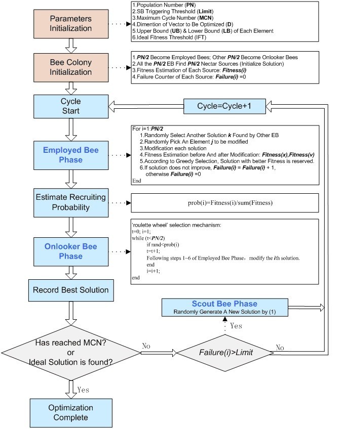

  

  Flowchart of ABC algorithm. It presents flowchart of original ABC algorithm. Colorful frames show the main phases, and detailed introduction are shown in the followed frame.

By above operations, ABC algorithm performs optimization. Nevertheless, in both EB and OB phases, the algorithm merely modify single element of the solution in each cycle. If the length of the solution vector D is large, it makes inefficiency improvement in each cycle. In [2], MR is proposed, which is a real number factor in [0, 1]. For element $x_i^{\left(j\right)}$ of solution i, a uniformly distributed random real number ($0\le R_i^{\left(j\right)}\le 1$) is produced. If $R_i^{\left(j\right)}\le MR$, element $x_i^{\left(j\right)}$ will be modified and others not. Moreover, if all $R_i^{\left(j\right)}$ are larger than MR, ensure at least one parameter being modified by original algorithm. Although this MR-ABC algorithm improves the convergence rate of basic algorithm to some extent, its robustness is not ideal according to testing by abundant experiments.

D-ABC algorithm

The original idea of ABC algorithm is to perform hierarchical optimization. Overall, global searching is performed by EB and local searching is implemented by OB. However, this idea is not prominent in traditional ABC algorithms, because the modifying extent of EB and OB is similar and relatively fixed. Dynamic modifying extent is more reasonable. To achieve more effective optimization, the activity of bees must be dynamic in different stages of the algorithm. Our idea is that global searching should be dominant in early cycles and local searching should be primary in the posterior cycles. This could be more consistent with actions of real bees: EB become main force in the initial, then more and more OB follow, they play the major role afterwards. Specifically, in early stages of optimization, audaciously modify more elements of $\overrightarrow{\text{x}}$ in EB phase. That makes the bees approaching better solution by a greater probability. Furthermore, OB become active in posterior stages, and they modify more elements of $\overrightarrow{\text{x}}$. That provides more opportunities to jump out of local optimal solution.

Consequently, we propose a dynamic ‘activity’ factor, and introduce it into modification operation of EB and OB phases. Adjust number of elements of the solution vector in each cycle. The ‘activity’ factor δ could be defined as following two forms by formulas (5) and (6), alternatively:

$$\delta =\Phi (C_c,MCN,D)$$

(5)

$$\delta =\Delta (F_c,IFT,D)$$

(6)

where C _c is current cycle number, , D is length of solution, F _c is current best fitness. The alternation of the two definitions depends on the termination condition of the algorithm. If using MCN to terminate the optimization, δ is defined as formula (5). And if IFT is employed, δ is defined as formula (6). δ_EB and δ_OB are ‘activity’ factor of EB and OB, respectively. Employ τ as the progress rate of the optimization, δ_EB and δ_OB subject to: (1) δ_EB grows with τ, when τ is not beyond half of total progress. ${\delta }_{\mathit{EB}}\in \left[0,1\right]$; (2) δ_OB grows with τ, when τ is beyond half of total progress.${\delta }_{\mathit{OB}}\in \left[0,1\right]$ . Explicit formulas could be determined according to specific problems. In this article, following scheme is suggested when utilize MCN as termination condition of the algorithm.

• (1) In early stages, for EB phase, δ_EB is defined as formula (7). It reduces with C _c increasing, and N_EB elements are randomly picked to be modified; For OB phase, MR method is recommended. Audacious global modification and conservative local modification are implemented.

  $$\begin{array}{c}\hfill EB\to N_{\mathit{EB}}=\left[{\delta }_{\mathit{EB}}·D\right]=\left[(1-\frac{C_c}{MCN})·D\right]\hfill \\ \hfill OB\to \text{MR}\begin{array}{}\end{array}\hfill \end{array}\}if{C}_c\le \frac{MCN}{2}$$

  (7)

• (2) In posterior stages, for EB phase, MR method is reused; For OB phase, δ_OB is defined as formula (8). It increases with C _c growing, and N_OB elements are randomly picked to be modified. Conservative global modification and audacious local modification are implemented.

  $$\begin{array}{c}\hfill EB\to \text{MR}\begin{array}{}\end{array}\hfill \\ \hfill OB\to N_{\mathit{OB}}=\left[{\delta }_{\mathit{OB}}·D\right]=\left[\frac{C_c}{MCN}·D\right]\hfill \end{array}\}\begin{array}{c}\hfill if\hfill \end{array}{C}_c>\frac{MCN}{2}$$

  (8)

Furthermore, D-ABC algorithm is closely to the length D of solution vector. When D is small, there is practically little difference between original ABC algorithm and D-ABC algorithm. And for larger D, the advantages of D-ABC algorithm are prominent on convergence rate and improving the quality of solutions.

Multi-parameters optimization of SVM-based soft-margin classifier

Introduction of SVM parameters optimization

As we all know, training soft-margin classifier is a constrained optimization problem as formula (9). l is number of samples, x _i is i th sample, and y _i is the label of sample i.

$$\begin{array}{l}\begin{array}{cc}\hfill \mathit{m}\mathit{i}\mathit{n}\mathit{i}\mathit{m}\mathit{i}\mathit{z}\mathit{e}\hfill & \hfill \frac{1}{2}\hfill \end{array}{\Vert w\Vert }^2+C\sum _{i=1}^l{\zeta }_i\\ subjectto{y}_i[w{x}_i+b]\ge 1-{\zeta }_i({\zeta }_i\ge 0,i=1,2,\dots ,l)\end{array}$$

(9)

It is a quadratic programming problem, which maximum the margin ($2/\Vert w\Vert$) when restricting the least classification error rate.

To solve unbalanced problem of training samples, ‘slack variable’ (ζ) and ‘cost’ factor (C) are introduced to process outlier samples and compromise the position of optimal separating hyper-plane. Large C indicates attaching importance to the loss of outliers of different classes. SVM needs to assign different C for each class. If these cost factors are not properly set, poor classification result will be obtained. However, experience-based setting is not robust. As a result, the multi-parameters optimizing problem needs to be solved, and parameters to be optimized will increase with number of class.

Additionally, parameters of kernel function of SVM need to be optimized. Solving (9) with Lagrange multiplier method, the separating classification function could be obtained as formulas (10) and (11), where α _i is Lagrange factor.

$$w=\sum _{i=1}^l\left({\alpha }_i{y}_i{x}_i\right)$$

(10)

$$g\left(x\right)=\sum _{i=1}^l{a}_{i}y<x_i,x>+b$$

(11)

When samples are linearly inseparable, SVM processes nonlinear problem as linear classification in high-dimensional, which is performed by kernel function as formula (12). Both number and type of parameters to be optimized are determined by the kernel function.

$$g\left(x\right)=\sum _{i=1}^l{a}_{i}yK(x_i,x,\gamma )+b$$

(12)

All above parameters to be optimized compose a vector $\overrightarrow{\text{x}}$, and the multi-parameters optimization problem is defined as (13):

$$\begin{array}{l}\begin{array}{cc}\hfill \text{maximize}\hfill & \hfill f\left(\overrightarrow{x}\right)\hfill \end{array}=f\left(\right\{C,\gamma ,q_1,q_{2,}\dots ,q_n\left\}\right)\\ \text{subject}\begin{array}{cc}\hfill \text{to}\hfill & \hfill \begin{array}{c}\hfill y_i[w{x}_i+b]\ge 1-\hfill \end{array}\hfill \end{array}{\zeta }_i\begin{array}{c}\hfill ({\zeta }_i\ge 0,i=1,2,\dots ,l)\hfill \end{array}\end{array}$$

(13)

where C is the cost factor, γ is the kernel parameter, and n is number of labels $q_j(j=1,2,\dots ,n)$, are weight parameters of each class, which set the cost factor C of class j to q, C. Moreover, to obtain creditable classification accuracy, ‘k-fold’ cross-validation is utilized for testing performance of SVM classifier. In our experiments, k is set to 10. Define the objective function $f\left(\overrightarrow{x}\right)$ as the average classification accuracy of ‘10-fold’ cross-validation as formula (14):

$$f\left(\overrightarrow{x}\right)=\sum _{m=1}^{k}Accurac{y}_m/k$$

(14)

Consequently, this problem could be solved by optimization algorithm. Owing to multiple parameters need to be optimized, our D-ABC algorithm is more suitable than traditional ABC algorithm. The flowchart of D-ABC algorithm based multi-parameters optimization is shown in Figure 2.

Figure 2

Flowchart of D-ABC algorithm-based multi-parameters optimization. It presents flowchart of optimizing process.

For a set of training samples, D-ABC algorithm modifies parameters vector $\overrightarrow{x}=\{C,\gamma ,q_1,q_{2,}\dots ,q_n\}$ cycle-by-cycle, and search best $\overrightarrow{x}$ for maximizing the classification accuracy.

Experiments

In this article, multi-class SVM-based soft-margin classifier is performed by C-support vector classification (C-SVC) toolbox. It is from LIBSVM toolbox supplied by Cheng and Lin [14]. The toolbox supply several typical kernel functions. Radial basis function is employed as kernel function in our experiments, and kernel parameter γ need to be optimized. For n-class classification, all parameters to be optimized and their range are presented in Table 1. Obviously, the length of vector $\overrightarrow{x}$ is D = n + 2. The dataset utilized for SVM training is as Table 2 shows. ‘Wine’ and ‘Image Segment’ are two typical testing dataset, which are widely used for testing SVM-based classifier. The two ‘building’ datasets are collected by us especially for multi-parameters optimization problem.

Table 1 Range of parameters to be optimized

Table 2 Dataset declaration

Performances of PSO algorithm, original ABC algorithm, MR-ABC algorithm, and D-ABC algorithm are compared for this optimization problem. All algorithms are coded under MATLAB 2011b. Main hardware configuration of our computer: Intel®Core(TM)2 Duo CPU P8400@2.26 GHz 2.27 GHz, 2.00 GB RAM.

According to principle of fair comparison: (1) corresponding initialization parameters are same set in these algorithms as Table 3 shows,the settings are according to [2]; (2) using same starting searching points to initialize the colony, as shown in Table 4 and Appendix. Mean value of 20 times running by different algorithms are collected as the final results for the four datasets, which are shown in Figures 3, 4, 5, and 6 and Table 4. Particularly, to verify the robustness of different algorithm, standard deviations of the 20 times run are given by Figures 7 and 8, for the two high-dimensional datasets.

Table 3 Parameters settings of different optimization algorithm

Table 4 Initial objection value of different datasets

Figure 3

Performance comparison of different algorithms for Dataset 1. X-axis presents number of cycles, and Y-axis indicates classification accuracy after optimized by different algorithms.

Figure 4

Performance comparison of different algorithms for Dataset 2. X-axis presents number of cycles, and Y-axis indicates classification accuracy after optimized by different algorithms.

Figure 5

Performance comparison of different algorithms for Dataset 3. X-axis presents number of cycles, and Y-axis indicates classification accuracy after optimized by different algorithms.

Figure 6

Performance comparison of different algorithms for Dataset 4. X-axis presents number of cycles, and Y-axis indicates classification accuracy after optimized by different algorithms.

Figure 7

Standard deviations of different algorithms for Dataset 3. X-axis presents number of cycles, and Y-axis indicates standard deviations of classification accuracy after optimized by different algorithms for 20 times runs.

Figure 8

Standard deviations of different algorithms for Dataset 4. X-axis presents number of cycles, and Y-axis indicates standard deviations of classification accuracy after optimized by different algorithms for 20 times runs.

Note that we choose measuring the convergence rate in cycle for following reasons: Generally, computational time of calling objection function is much larger than other parts of ABC algorithm, particularly when our objection function includes multiple times SVM training. The SVM training takes more than much time, and in each cycle, the code of objection function will be called many times (same times in each cycle for different algorithm, and times is determined by parameter PN). Objection function calling occupies more than 90% computational time of both original ABC algorithm and modified ones (for instance, for dataset 4, about 22.3 s are cost by running D-ABC algorithm for each cycle, 21.7 s for MR-ABC algorithm, and 20.5 s for original ABC algorithm. It is obviously that objection function cost most time in each cycle). Moreover, every time the objection function is called, the solution is modified. Therefore, it is more reasonable measuring the convergence rate in cycle than in time. On the contrary, if measuring the convergence rate in specified computational time, each solution might be modified different times, which could be unfair.

As is shown in Figure 3, for dataset 1, D-ABC algorithm rapidly find a solution $\overrightarrow{\text{x}}$, with which SVM could best training the data and obtain a classification accuracy of 98.88 %, while original ABC algorithm and MR-ABC obtain that solution slowly. Though PSO algorithm has a good convergence rate, it could not get an ideal solution. As is shown in Figure 4, for dataset 2, similarly, compared with original ABC algorithm and MR-ABC, D-ABC algorithm performs better convergence rate and obtains higher classification accuracy, and the improvement is more obvious than dataset 1. PSO algorithm still converges fast but an unsatisfactory solution. By contrast, D-ABC algorithm obtains a classification accuracy of 92.38 %.

The results above have demonstrated the advantages of D-ABC algorithm for lower dimension of parameter-vector like datasets 1 and 2. Furthermore, datasets 3 and 4 are collected for testing optimization of higher dimensional $\overrightarrow{\text{x}}$. As is shown in Figures 5, 6, and Table 5, similar conclusions could be obtained that D-ABC algorithm has certain advantages over other algorithms, which lead to greater improvement on convergence rate and quality of solution, especially when D is larger. Moreover, standard deviations (of 20 times run) for the two groups of datasets are shown in Figures 7 and 8, respectively. The curves illustrate the standard deviations of objection function in different optimizing cycles, and the relatively lower standard deviations have been obtained by D-ABC algorithm for both datasets 3 and 4, which indicates that D-ABC algorithm has good robustness.

Table 5 Best solution obtained by different optimization algorithms

Conclusion and discussion

In this article, two parts of work have been studied. First, D-ABC algorithm is introduced to improve the disadvantages of traditional ABC algorithms: poor convergence rate and local optimizing. Second, D-ABC algorithm is utilized for multi-parameters optimization of SVM classifier. Experiments results demonstrate that D-ABC algorithm is in many ways superior to traditional ABC algorithms. It effectively ameliorates the convergence rate and local optimum. Typically, for multi-parameters optimization, when length D of vector (to be optimized) is larger, our study has provided substantial evidence for the advantages of D-ABC algorithm on quality of solution and convergence rate. When D-ABC algorithm is employed for optimizing multi-parameters of SVM-based soft-margin classifier, great improvement is obtained on performance of the classifier. Moreover, the robustness of D-ABC algorithm is proofed. Furthermore, the idea of D-ABC algorithm could be associated with other modified ABC algorithms, whose modification is on other phase of original ABC algorithm, and it might further improve traditional ABC algorithm in future work.

Appendix

The starting searching points of the four group of experiments are tabulated in Tables 6, 7, 8, and 9.

Table 6 The initial colony of dataset 1

Table 7 The initial colony of dataset 2

Table 8 The initial colony of dataset 3

Table 9 The initial colony of dataset 4

References

Karaboga D: An Idea Based on Honey Bee Swarm for Numerical Optimization. Technical Report, TR06. Erciyes University Press, Erciyes; 2005.
Karaboga D, Akay B: A modified artificial bee colony (ABC) algorithm for constrained optimization problems. Appl. Soft Comput. 2010, 11(3):3021-3031. 10.1016/j.asoc.2010.12.001
Akay B, Karaboga D: A modified artificial bee colony algorithm for real-parameter optimization. Inf. Sci 2012, 192: 120-142. 10.1016/j.ins.2010.07.015
Singh A: An artificial bee colony algorithm for the leaf-constrained minimum spanning tree problem. Appl. Soft Comput. 2010, 9(2):625-631. 10.1016/j.asoc.2008.09.001
Bao L, Zeng J: Comparison and analysis of the selection mechanism in the artificial bee colony algorithm. 1st edition. Paper presented at Ninth International Conference on Hybrid Intelligent Systems (HIS '09), Shenyang, LiaoNing, China; 2009:411-416.
Parpinelli RS, Benitez CMV, Lopes HS: Parallel approaches for the artificial bee colony algorithm, handbook of swarm intelligence: concepts. Princ. Appl. 2011, 8: 329.
Haijun D, Qingxian F: Artificial bee colony algorithm based on Boltzmann selection policy. Comput. Eng. Appl. 2009, 45(31):53-55.
Tsai P, Pan J, Liao B, Chu S: Interactive artificial bee colony (IABC) optimization. ISI2008, Taipei Taiwan; 2008.
Akbari R, Mohammadi A, Ziarati K: A novel bee swarm optimization algorithm for numerical function optimization. Commun. Nonlinear Sci. Numer. Simul 2010, 15: 3142-3155. 10.1016/j.cnsns.2009.11.003
Cortes C, Vapnik V: Support-vector networks. Mach. Learn 1995, 20: 273-297. 10.1007/BF00994018
Samadzadegan F, Soleymani A, Abbaspour RA: Evaluation of Genetic Algorithms for tuning SVM parameters in multi-class problems. Paper presented at 11th International Symposium on Computational Intelligence and Informatics (CINTI), Budapest; 2010:323-328.
Yang L, Wang HT: Classification based on particle swarm optimization for least square support vector machines training. Paper presented at Third International Symposium on Intelligent Information Technology and Security Informatics (IITSI), Jinggangshan; 2010:246-249.
Hsieh TJ, Yeh WC: Knowledge discovery employing grid scheme least squares support vector machines based on orthogonal design bee colony algorithm. IEEE Trans. Syst. Man Cybern. B: Cybernetics 2011, 41(5):1-15. 10.1109/TSMCB.2011.2116007
Chang CC, Lin CJ: LIBSVM: a library for support vector machines. ACM Trans. Intell. Syst. Technol. (TIST) 2011, 2(3):27. 10.1145/1961189.1961199
Author information
Authors and Affiliations
Corresponding author
Additional information
Competing interests
The authors declare that they have no competing interests.
Authors’ original submitted files for images
Below are the links to the authors’ original submitted files for images.
Rights and permissions
Open Access This article is distributed under the terms of the Creative Commons Attribution 2.0 International License (https://creativecommons.org/licenses/by/2.0), which permits unrestricted use, distribution, and reproduction in any medium, provided the original work is properly cited.
About this article
Cite this article
Yan, Y., Zhang, Y. & Gao, F. Dynamic artificial bee colony algorithm for multi-parameters optimization of support vector machine-based soft-margin classifier. EURASIP J. Adv. Signal Process. 2012, 160 (2012). https://doi.org/10.1186/1687-6180-2012-160
Received:
Accepted:
Published:
DOI: https://doi.org/10.1186/1687-6180-2012-160