- Research
- Open access
- Published:
On the conditions for valid objective functions in blind separation of independent and dependent sources
EURASIP Journal on Advances in Signal Processing volume 2012, Article number: 255 (2012)
Abstract
It is well known that independent sources can be blindly detected and separated, one by one, from linear mixtures by identifying local extrema of certain objective functions (contrasts), like negentropy, non-Gaussianity (NG) measures, kurtosis, etc. It was also suggested by Donoho in 1981, and verified in practice by Caiafa et al., that some of these measures remain useful for particular cases with dependent sources, but not much work has been done in this respect and a rigorous theoretical ground still lacks. In this article, it is shown that, if a specific type of pairwise dependence among sources exists, called linear conditional expectation (LCE) law, then a family of objective functions are valid for their separation. Interestingly, this particular type of dependence arises in modeling material abundances in the spectral unmixing problem of remote sensed images. In this study, a theoretical novel approach is used to analyze Shannon entropy (SE), NG measure and absolute smoments of arbitrarily order β, i.e. generic absolute moments for the separation of sources allowing them to be dependent. We provide theoretical results that show the conditions under which sources are isolated by searching for a maximum or a minimum. Also, simple and efficient algorithms based on Parzen windows estimations of probability density functions and Newton–Raphson iterations are proposed for the separation of dependent or independent sources. A set of simulation results on synthetic data and an application to the blind spectral unmixing problem are provided in order to validate our theoretical results and compare these algorithms against FastICA and a very recently proposed algorithm for dependent sources, the bounded component analysis algorithm. It is shown that, for dependent sources verifying the LCE law, the NG measure provides the best separation results.
Introduction
In signal processing, a generic problem is how to separate signals that are linearly combined in the measurements. Blind source separation (BSS) consists on the task of isolating n sources from a set of m linear mixtures:
where is a column vector containing the mixtures (observed measurements), is a column vector containing the unknown source signals (sources) and is the unknown mixing matrix containing the mixing coefficients. The parameter t is an index that can be related to the position in time or space (pixel index) depending on the application. The model of Equation (1) is commonly referred as the noiseless instantaneous mixing model.
When sources are statistically independent and m ≥ n (overdetermined case), the problem is well posed in the sense that sources can be identified up to some unimportant indeterminacies[1]. This result allowed the development of a sort of independent component analysis (ICA) algorithms which were successfully and widely used in engineering problems[2–4]. Many criteria have been proposed in the context of ICA, for example, it is known that sources can be detected by identifying the local minima of the SE, in the space of the mixing parameters, keeping the variance constant because of a classic result from information theory: the entropy of a sum of independent variables is larger than the entropy of individual variables[1, 3, 5–7]. More generally, Comon[1] has introduced the definition of contrasts for ICA, i.e. objective functions such that their global maxima corresponds to the separation of all sources. Besides negentropy (negative SE), other contrasts have been proposed for ICA as it is the case of higher order cumulants for which fourth order cumulant is a particular case[3, 8–10], the convex perimeter for bounded sources[11], L2-distance non-Gaussianity (NG) measure[12], least absolute end-point (LAE)[13], and others. For an up to date review of existing algorithms for ICA, the reader may refer to[2].
Unlike in the ICA case, the separation of dependent sources or dependent component analysis (DCA), has not been fully studied in the past and showed more difficulties. Hyvärinen & Hoyer[14] have proposed independent subspace analysis (ISA) as an extension of ICA where components in different subspaces are assumed independent whereas components in the same subspace have dependencies. When the sources and the mixing matrix are restricted to be non-negative, the problem can be seen as a non-negative matrix factorization (NMF) problem for which many algorithms have been developed[15]. However, NMF suffers from non-uniqueness of the solutions and the separation is not granted if not additional constraints are assumed, for example, by imposing sparsity of sources[16, 17]. Bedini et al.[18] have developed algorithms for the separation of correlated sources found in astrophysical applications based on multiple-lag data covariance matrices, i.e. by exploiting the time structure of sources. In[12, 19], an algorithm called MaxNG based on the maximization of a NG measure was proposed and tested on dependent sources extracted from remote sensed images. In[20, 21], some DCA methods were tested on astrophysical sources. Cruces[11] proposed bounded component analysis (BCA) as an alternative method for BSS which relies on the bounded support of sources. In BCA, the separation is granted when the convex hull of the sources domain can be written as the cartesian product of the convex hulls of the individual source supports which is a very restrictive assumption. Recently, Eldogar[22] showed that a particular type of dependent sources generated according with a copula-t distribution are perfectly separated by BCA for a wide range of the correlation coefficient.
In all the previously mentioned DCA methods, when the independence assumption is relaxed, the success of the separation relies on alternative, and usually very restrictive conditions on sources. Moreover, it was suggested in[23], and verified in practice in[12, 19, 24], that some measures used in ICA, such as negentropy, NG and kurtosis, remain useful for particular cases with dependent sources, but not much work has been done in this respect and a rigorous theoretical ground still lacks.
In this work, we propose a unified theoretical framework to study the capability of any objective function to detect each of the sources as a local maximum (or minimum) in the space of coefficients. From our analysis, it turns out that many new objective functions can be proposed owing this property if a particular type of dependence is verified among sources. In particular, we analyze generic absolute (GA) moments, SE and NG measure as valid objective functions. We introduce simple and efficient algorithms for the separation of sources using Parzen windows estimations of pdfs and Newton–Raphson (N–R) iteration. We analyze the performance of these measures and compare them against FastICA and BCA algorithm.
This article is organized as follows: in Section 2, the theoretical aspects are introduced followed by detailed analysis of the independent sources case (Section 3) and the dependent sources case (Section 4); in Section 5, using this theory, a set of particular cases are rigorously analyzed and illustrated by simulations; in Section 6, algorithms for source separation with n = 2 sources are derived by using Parzen windows estimation of pdfs and N–R iterative method; in Section 7, several simulation experiments are presented showing the performance of the proposed algorithms and comparing them against FastICA and BCA; finally, in Section 8, the main conclusions of this work and a discussion about our results is included.
Notation and assumptions
We use capital letters to denote random variables, for example, S1, S2,…, S n are the random variables associated to the sources which have a joint probability density function (pdf) denoted by. Obviously, when sources are independent, the joint pdf factorizes, i.e.
where is called the marginal pdf of variable S i . In this work, we are also interested in the case of having dependent sources where such a factorization of the joint pdf does not exist.
We also define the conditional pdf of a random variable S1 given that S2 = x as follows:. Accordingly, we define the first and second order conditional expectations as follows: and. In the case of having only two sources, we can simplify the notation by using E[S1|x] ≡ E[S1|S2 = x] and. Since conditioned expectations are functions of x, we use the following simplified notation: and.
In several parts of this article, when we apply the differentiation operator under the integral sign, i.e. we will assume that the function g(x, τ) is sufficiently nicely behaved in order to allow this operation. Basically, we assume that g(x, τ) and are continuous for x in the range of integration and there are upper bounds |g(x, τ)| ≤ A(x) and independent of τ such that the integrals ∫A(x)dx, ∫ B(x)dx do exist.
A motivation for this work: the blind spectral unmixing problem
Blind spectral unmixing is a specific application of BSS to the analysis of hyper-spectral remote sensed images. In this case, it is known that, at any fixed pixel, the linear mixing model of Equation (1) is valid. The vector of mixtures x represents the sensor measurements at different wavelengths, matrix A contains in its columns the spectral signatures of the endmembers (materials) existing in the covered area and vector s contains the endmember fractional abundances at the given pixel[25]. When the spectral signatures are unknown this is a blind problem and the objective is to estimate both, matrix A and the endmember fractional abundances s.
Most of the existing spectral unmixing algorithms exploit geometrical concepts by using the fact that, due to the linear mixing equation, the mixed pixels have to lie inside the convex hull of the endmembers. This convex hull forms a simplex in the spectral space, with the endmembers as spanning vertices. Some algorithms then try to look for the largest volume embedded simplex (e.g. simplex growing algorithm (SGA)[26], simplex-projection unmixing (SPU)[27]) or try to identify extreme points in the data cloud (e.g. vertex component analysis (VCA)[28]). Other recently proposed methods are based on the NMF with sparsity assumptions (e.g. S-measure constrained NMF algorithm (NMF-SMC)[29]).
As a BSS problem, sources in the blind spectral unmixing problem are clearly not independent since they are related to fractional abundances, in fact, they are constrained to sum up to one, i.e.. Additionally, in order to avoid scale indeterminacy and remove constant values, we have to work with normalized sources S i , i.e. where μ i and σ i are the mean and standard deviation associated to source i. Under these conditions, the blind spectral unmixing task can be approached by solving a BSS problem with the additional constraint[19]:
with
The dependence between any pair of normalized sources can be characterized, for example, by the conditional expectations E[ S i |S j ] and E[ S j |S i ] (i ≠ j). Clearly, when sources are independent, we have E[ S i |S j ] = E S i = 0. On the other hand, when sources are dependent the conditional expectation E[ S i |S j ] (i ≠ j) is a function of S j . We can try, to determine these functions in order to satisfy Equation (3). By applying the conditional expectation to this equation with respect to S i (i = 1, 2,…, n) we obtain a system of n equations with n2 − n unknown (the conditional expectations E[ S i |S j ] ∀ i ≠ j). Thus, for n ≥ 2 there is not a unique choice of the conditional expectations. Then, we have to obtain this information from the observation of real data. In[19], it was shown that hyper-spectral data can be well modeled as having linear conditional expectations (LCEs), i.e. E[ S i |S j ] = a S j + b (see[19]). The following theorem provides us the values of the constants a and b.
Theorem 1
( [[19]], Theorem 3):Given a pair of dependent normalized sources S i , S j , if the conditional expectation E[ S i |S j ] is linear in S j , that is E[ S i |S j ] = a S j + b, then a = E[ S i S j ] and b = 0.
In other words, in the blind spectral unmixing problem, the normalized sources can be modeled as verifying the following condition:
which is called the LCE law.
As we demonstrate in this article, when this particular type of dependence between sources is valid, their separation from linear mixtures can be obtained by maximizing (or minimizing) different types of objective functions.
Relationship with previous works and new contributions
In[12], we have proposed the Parzen based NG measure and developed the MaxNG algorithm, a DCA method which showed to be useful to separate dependent sources extracted from images and also astrophysical dependent sources[20], outperforming classical ICA algorithms. However, in those articles the NG measure was not rigorously justified. Later, in[19], the NG measure was proposed as a solution for the blind spectral unmixing problem and a partial theoretical justification was given in terms of the LCE condition (guarantee of local extremum). In[24], we reported the results obtained by extending our method to other measures of NG such as Negentropy, and moment based measures, and applying them to synthetic and real datasets in the blind spectral unmixing problem context. However, a complete theoretical foundation was still lacking and several questions arose from those experimental results, for example: (1) why kurtosis based measure failed to separate one specific type of dependent sources? or (2) given a particular measure, how to determine if it can be used for the separation of sources by local maximization or minimization?, and (3) on which conditions on sources the separation can be granted? In the present manuscript, we present a unified theoretical framework for the study of different measures for separation of independent and dependent sources verifying the LCE condition. The main contribution of this manuscript is to fill the gaps existing among previous works and give rigorous theoretical answers to the above open questions. In particular, it is shown that the kurtosis based measure (i.e. GA moment with β = 4) has zero second order derivative for the constrained dependent sources, which makes it useless for the separation as our empirical results showed in[24]. We also provide a precise condition (see Equation (33)) that establishes whether independent sources are separated by maximizing or minimizing the corresponding GA moment μ β (θ). On the other side, for dependent sources, it is necessary to know the second order conditional expectations, i.e.. Another contribution of the present article is a new algorithm based on a N–R search for local extrema which has quadratic convergence, i.e. being much faster than the algorithms proposed in[12, 19, 20] which used a steepest ascend method with fixed update step. Additionally, in the present manuscript we compare our algorithms against a recently proposed DCA algorithm, namely, the BCA[22], one state-of-the-art algorithm for DCA.
Detection of sources by maximizing or minimizing objective functions
In this article, we focus only on sequential methods, also known as deflation methods, that extract normalized sources one after another by searching for local extrema of a predefined objective function. This simple idea was already used in the ICA context[2, 3] and can be introduced as follows. When the matrix A in Equation (1) is full-column rank, the sources can be expressed as a linear combination of the mixtures by premultiplying Equation (1) with a pseudo inverse matrix such as the case of the Moore–Penrose pseudoinverse A†, i.e.
Since matrix A is unknown, a reasonable strategy could be to search in the space of coefficients, for those points which correspond to each one of the sources. In other words, if we denote by S i the random variable associated to the source then we need to analyze the behavior of the mixture random variable X defined as:
We say that variable S i is separated from the mixture when all coefficients are zero except α i , i.e. α i = 1 and α j = 0 for every j ≠ i. Here we arrive at the main question we want to answer in this article: how can we discriminate between a single source compared to any linear combination of two or more sources?
We introduce some important objective functions that allow us to answer this question. Any valid candidate for an objective function should involve the pdf of the mixture f X (x) which depends on the mixture coefficients α i . In particular we consider the SE:
the NG measure defined as follows[12, 19]:
where, and the GA moment of order β which is defined as follows:
The SE is a well known measure already used in ICA, on the other side the GA moment was not used before for BSS except in the particular case when β = 4 which is closely related with the kurtosis[3, 9]. In fact, kurtosis is defined as. In this sense, our analysis generalizes existing ICA methods providing insightful interpretations of the results. Note that, for β = 2 we obtain the second order moment of the variable which, in our case is fixed to μ2 = 1. But we can choose any order of moment β provided that the integral in Equation (9) exists. In the following section we prove that these objective functions are valid for ICA.
Independent sources case
Let us focus on Equation (6) and analyze wether it is possible to isolate a source S i from the rest by only looking at the statistical behavior of the mixture variable X, i.e. by studying how the pdf f X (x;α) varies according to the mixing parameters in the vector α = (α1, α2, …, α n ). For the ease of the presentation we start with the analysis of the two independent sources case. Since we have to generate all possible mixtures of two independent sources maintaining the variance constant, we use the following parameterization: X = α1(θ)S1 + α2(θ)S2 with α1(θ) = cos(θ) and α2(θ) = sin(θ) which means that the separation is obtained at θ = kΠ / 2 (k = 0, ± 1, ± 2,…) (ignoring scaling ambiguity). We first introduce a new result characterizing the pdf of a mixture of independent random variables as a function of the mixing parameter θ, i.e. f X (x;θ).
Lemma 1
(Two independent sources case): Given two zero-mean and unit-variance independent source variables S1and S 2 , the pdf f X (x;θ) of the mixture variable X = α1(θ)S1 + α2(θ)S2with α1(θ) = cos(θ) and α(θ) = sin(θ), has zero-derivative with respect to θ for every x at θ = kΠ / 2 (k = 0, ±1, ±2,…), i.e.
Proof
Let us prove first the zero-derivative condition (maximum or minimum) at θ = Π / 2 (α0 = (α1, α2) = (0, 1)) which corresponds to the separation of source S2. In the neighborhood of α0, i.e. α = α0 + δ, we can write the pdf of the mixture as the convolution:
By using the chain rule of derivatives we obtain
We compute the partial derivatives in the last equation evaluated at α1=0 and α2=1 and, by inserting the derivative operator inside the integral, we obtain:
Now, taking into account that and, and using Equations (13) and (14) into Equation (12), we arrive at
for every x. Using a similar procedure but working in a neighbouhood of α0=(α1,α2)=(1,0), i.e. by considering instead of Equation (11), we can prove the zero-derivative condition at θ=0, which corresponds to the separation of source S1. Finally, it is easy to see that the zero-derivative condition also holds for any integer multiple of Π/2, because the resulting mixture becomes ±S1or ±S2and the same reasoning used before applies. Thus, the zero-derivative condition is valid for every x at θ=kΠ/2 (k=0,±1,±2,…) as claimed by this lemma. □
In Figure1, a graphical interpretation of this lemma is shown in terms of the shape of the pdf for a mixture of two independent sub-Gaussian variables at θ0=Π/2 and θ=θ0±δθ.

pdf for the mixture variable X =α 1 (θ)S 1 + α 2 (θ)S 2 with sub-Gaussian sources at θ 0 =Π/ 2 (left) and at θ=θ 0 ±δθ (right). Note that, when θ=Π/2 the pdf corresponds to the source S2, on the other side, when a perturbation on the mixing parameter θ is considered, i.e. θ=θ0±δθ, a pdf with a shape closer to the Gaussian one is obtained. It is also noted that in the intervals () the pdf f X (x;θ) attains its minimum (maximum) at θ=Π/2.
In the following, using this fundamental property of independent variables (Lemma 1), we can easily prove that g SE (θ) and μ β (θ) have local extrema at the desirable separation points, i.e., for k∈.
Theorem 2
Local extrema of SE (independent sources case): Given two zero-mean and unit-norm source variables S i (i=1,2), the SE (g SE (θ)) of the mixture variable X=cos(θ)S1 + sin(θ)S2, has local extrema at θ=kΠ/2 (k∈).
Proof
As in the proof of Lemma 1, here it suffices to prove that the derivative of the SE, with respect to the parameter θ, vanishes at θ=Π/2. From the definition of SE in Equation (7), if we take its derivative with respect to θ we have:
Now, using Lemma 1 we see that the derivative of the pdf is zero at θ=Π/2 for every x and therefore we conclude that. □
Theorem 3
Local extrema of the GA moment measure (independent sources case):
Given two zero-mean and unit-norm source variables S i (i=1,2), the GA moment of order β, μ β (θ) of the mixture variable X=cos(θ)S1 + sin(θ)S2, has local extrema at θ=kΠ/2 (k∈).
Proof
We need to prove that the derivative of Equation (9), with respect to the parameter θ, is zero at θ=Π/2. If we take the derivative of this equation we obtain:
where, by using the Lemma 1, we see that. □
It is interesting to note that, our Theorem 3 shows that local extrema are found at the desirable locations for any chosen value of parameter β.
In[19], it was shown that the NG measure defined in Equation (8) has also local extrema at the separation points. Moreover, it is clear that, by using the same line of reasoning we can prove the existence of local extrema in many other objective functionals as, for example, for the case of Renyi entropy which was already proposed and studied for ICA[6, 7].
It is important to note that, a local extremum at (α1α2)=(0,1) is a necessary condition to separate source S2but it is not a sufficient condition. The existence of local extrema which do not correspond to a separation of sources, also known as mixing local extrema or spurious local extrema, was a topic of research in the ICA setting. Moreover, some theoretical results are available showing the existence of spurious local minima for the Entropy measure when sources has multimodal distributions[30, 31]. Vrins and Verleysen[32] have shown that the kurtosis-based contrast functions are more robust than the information theoretic ones when the source distributions are multimodal.
Relaxing independence: DCA
In the previous section, we have shown that Lemma 1 suffices to guarantee the validity of the SE, the GA moment and the NG measure as objective functions for ICA. We are interested now to look at the problem of separation of potentially dependent sources. Then, a natural question raises here: what kind of dependence should have the sources in order to guarantee the same behavior of the pdf as in the ICA scenario? The following result provides a necessary and sufficient condition.
Lemma 2 (n dependent sources case)
Given a set of zero-mean and unit-variance source variables S i (i=1,2,…,n) the pdf f X (x;α) of the mixture variable X=α1S1 + α2S2 + ⋯ + α n S n , constrained to the case of having unit-variance E[X2]=1, has local extrema for every x at the separation points (α k =1 and α i =0 for all i≠k) iff the LCE law defined in Equation (4) holds.
Proof
Here it is only necessary to prove the local extrema condition (maximum or minimum) for only one point so we arbitrarily choose the case α n =1 and α i =0 for all i≠n. In this case, in the neighborhood of α0=(0,0,…,1), i.e. α=α0 + δ, we can write the pdf of the mixture as follows:
Following the Lagrangean method, the condition for the existence of a local extrema point at α=α0 under the unit-variance constraint is as follows:
with
where λ is the Lagrange multiplier and ρ ik =E[S i S k ] is the correlation coefficient between sources i and k.
Now, we take the derivatives of the pdf in Equation (18) with respect to the coefficients α i with i=1,2,…,n−1 which, evaluated at α=α0give:
Similarly, the derivative of the pdf in Equation (18) with respect to the coefficient α n is:
Using Equations (20), (21) and (22) in Equation (19) we obtain the following set of conditions:
The last equation determines the Lagrange multiplier, i.e. and, by inserting it into (23) we arrive to the desired condition:
□
It is important to note that the LCE condition is also valid for the particular case of independent sources, i.e. E[S1|S2=s2]=E[S1]=0 and ρ=0. In Figure2, some examples of sources are given indicating whether they follow or not the LCE law.

Scatter plots for three examples of sources with estimations of the conditional expectation E [S 1 |S 2 ] and the linear regression given by ρS 2 : (a) corresponds to a pair of independent sources (sub-Gaussian); (b) corresponds to a pair of dependent sources with negative correlation following the model of abundances in spectral unmixing problem (constrained case); and (c) shows a pair of dependent sources generated using a Copula-t distribution with correlation ρ = 0.8. In (a) and (b) the LCE condition holds while in (c) it is only approximately verified.
Before proceeding with our additional results, we have to solve a technical problem because, as our sources are now dependent they are allowed to be correlated, thus the parameterization X=cos(θ)S1 + sin(θ)S2 does not longer preserve the variance of the mixture variable X. Let us consider the general linear mixture X=α1S1 + α2S2, if we are constrained to the unit-variance case E[X2]=1, then, where we used ρ=E[S1S2] to denote the correlation coefficient between sources. Then, the following parameterization preserves the variance and uses only one parameter τ:
The following results can be considered as generalizations of Theorems 2 and 3 to the case of two dependent sources.
Theorem 4
Local Extrema of SE (general case): Given two zero-mean and unit-norm source variables S i (i=1,2) following the LCE law with respect to S2, the SE of the mixture variable X=α1S1 + α2S2constrained to the unit-variance case E[X2]=1, has a local extremum at (α1,α2)=(0,1).
Proof
The proof can be obtained identically to the proof of Theorem 2, taking into account the parameterization (26) and using the fact that the LCE condition implies the existence of local extrema of the pdf as stated by Lemma 2. □
Theorem 5
Local extrema of the GA moment (general case): Given two zero-mean and unit-norm source variables S i (i=1,2) following the LCE law with respect to S2, the GA moment of order β of the mixture variable X=α1S1 + α2S2, constrained to the unit-variance case E[X2]=1, has a local extremum at (α1,α2)=(0,1).
Proof
The proof can be obtained identically to the proof of Theorem 3, taking into account the parameterization (26) and using the fact that the LCE condition implies the existed of the local extrema of the pdf as stated by Lemma 2 □
Detailed analysis of SE and GA moment s
In previous sections, we proved that some objective functions applied to a unit-variance mixture of sources verifying the LCE law, have local extrema when only one of the coefficients is non-zero, which means that we can separate those sources by searching for local extrema. Nevertheless, a more detailed analysis is required in order to determine if each local extremum corresponds to a maximum or a minimum.
Here, we compute the second order derivative of the objective function with respect to τ for the special cases of the SE and GA moments of order β. As we will show, the condition of a maximum or minimum depends on the second order conditional expectation of sources and on their marginal pdfs. First we need to compute the second order derivative of the pdf with respect to the parameter τ which is as follows (its derivation is included in Appendix 1):
We note that the second order derivative explicitly depends on the second order conditional expectation and the marginal pdf.
Using this result, we are able to obtain the second order derivatives of the objective function as follows:
-
(1)
SE measure: to obtain the second order derivative of SE we take the derivative of Equation (16) with respect to the parameter τ arriving at:
(28)and, by using Equation (27) in the last equation and taking into account that the LCE law holds, i.e. E[S1|x]=ρx, we obtain (see its derivation in Appendix 2):
(29) -
(2)
GA moment: To compute the second order derivative of the GA moment we need to take the derivative of Equation (17) with respect to the parameter τ reaching to:
(30)Again, by using Equation (27) into the last equation and using the LCE law we obtain (see its derivation in Appendix 3):
(31)which is valid only when the integral exists.
Some particular cases
In this section, we analyze selected examples to illustrate our theoretical results applied to different types of independent and dependent sources.
-
(1)
Independent sources: Let us consider the simplest case of having two independent sources S 1 and S 2. We see that the LCE law (Equation (4)) holds since ρ=0 and E S 1|S 2=s 2=E S 1=0 which means that SE, GA moment and NG measure have a local extrema at τ=0 using the parameterization of Equation (26). Additionally, we note that the second order conditional expectation is and then the second order derivative of SE using Equation (29) becomes:
(32)which is always greater than zero except for the Gaussian distribution for which is equal to zero (see for example[33], p. 23). This confirms the fact that, at the separation point, we have a local minimum of the SE.Now, using Equation (31) we evaluate the second order derivative of the GA moment which is
(33)Let us now analyze different cases corresponding to different values of β. For example, if we consider the fourth order moment case (β=4), we obtain which means that, for sources with β4>3 (super-Gaussian) the fourth order moment of the mixture has a minimum at τ=0. On the other hand, for sources with μ4<3 (sub-Gaussian), a maximum of the fourth order moment of the mixture is found. More interestingly, we can evaluate any arbitrarily order β and Equation (33) will tell us if we need to search for a maximum or a minimum to attain the separation.
-
(2)
Uncorrelated but dependent sources: We consider here two sources S 1 and S 2 generated as follows: S 1=N 1 N 2and S 2=N 2, where N 1 and N 2 are independent non-Gaussian random variables with E[N 1]=E[N 2]=0 and . We see that S 1 and S 2 are highly dependent but are uncorrelated because . The first order conditional expectation is zero, i.e. E[S 1|S 2=s 2]=E[N 1]s 2=0. We also compute the second order conditional expectation which is . Then, by using Equation (29), the second order derivative of SE at τ=0 becomes:
(34)It is interesting to note that SE could have a maximum at τ=0 if the integral in the last equation is smaller than three as in the case of our example in Figure3d.
Figure 3 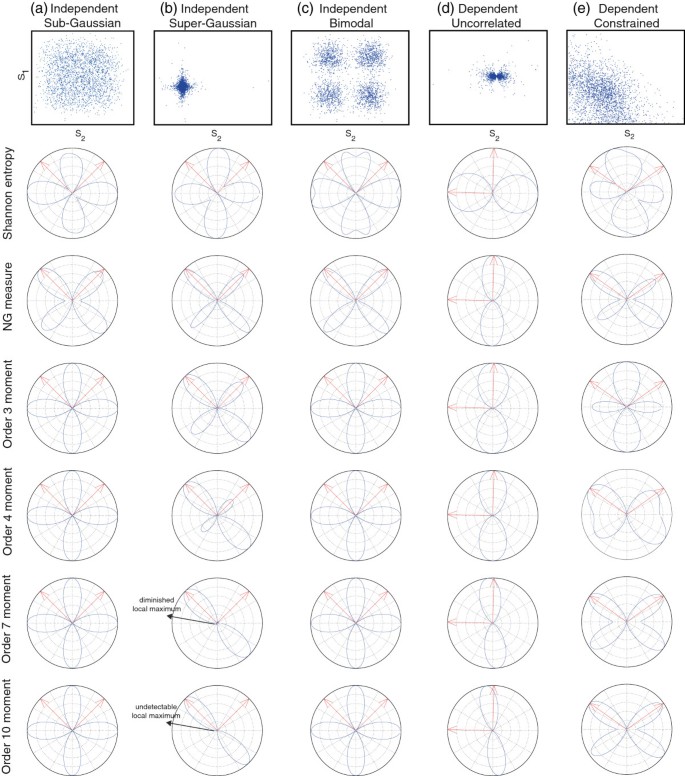
Computation of SE, NG measure and GA moments for different types of independent and dependent sources S 1 and S 2 . After a de-correlation step (whitening) the measures are computed using the polar parameterization y(θ)=cos(θ)X1 + sin(θ)X2where X1and X2are the whitened variables. The corresponding scatter plots are shown in the 1st row. The position of theoretical positions (in polar coordinates) are shown as red arrows. The measures were normalized in order to cover the range [0,1]. We used signals with a total number of samples T=106but we used only a subset of 10,000 samples to compute SE and NG measure to avoid the extremely high computational demand. For the generation of sub-Gaussian and super-Gaussian sources we used the transformation sinh−1(x) and sinh(x) applied to a Gaussian variable x, respectively.
Regarding the GA moment, for these sources, Equation (31) becomes:
(35)and we conclude that we have a minimum at the separation point () for every β>2.
-
(3)
A simplified model for material abundances in spectral unmixing (dependent sources): A simple model to generate a special type of sources which are dependent, correlated and constrained to have their sum constant is as follows [19]. First, we generate P>2 independent, nonnegative random variables N 1 N 2,…,N P ; then, we define the following random variables: , for i=1,2,…,P. We note that these signals meet the constraint as in the spectral unmixing application. Now, we define our sources by normalizing two of these constrained sources, i.e.: , i=1,2. It is not hard to prove that these sources meet the LCE law since E S 1 S 2=ρ=−1/(P−1) and E S 1|S 2=s 2=ρ s 2=−1/(P−1)s 2. Additionally, It is not difficult to prove that, for this particular type of sources we have constant GA moment of order β=4 which makes it not suitable as an objective function for this case. This behavior was already observed in [24] but not theoretical explanation was available until now. In Section 7.3, we generate data and test ICA/DCA algorithms using a more realistic model for material abundances in hyperspectral images by computing directly the material percentages per pixel in a real image.

In order to illustrate these theoretical results, in Figure3, plots for SE, the NG measure, and GA moments with several values of β, are shown for the following types of datasets using a sample size of T=106 (except for SE and NG for which we used T=104): (a) Independent sub-Gaussian sources, generated by applying the function sinh(u)−1 to zero-mean Gaussian independent signals; (b) Independent super-Gaussian sources, generated by applying the function sinh(u) to zero-mean Gaussian independent signals; (c) Independent bimodal sources, where each of the independent sources were generated by mixing two Gaussians with (μ1,σ1)=(0. 5,0. 2) and (μ2,σ2)=(−0. 5,0. 2), respectively; (d) Dependent uncorrelated sources, generated by using and where were generated as independent zero-mean uniform distributions; and (e) Dependent constrained sources, generated by using with i=1,2, where signals (p=1,2,…y,4) were generated using independent uniform distributions in [0,1].
We see that for the cases (a), (b), (c) and (e), the separation of each source is attained at the minima of the SE and the maxima of the NG measure. Interestingly, sources in case (d) (dependent and correlated) shows that one of the sources is detected at one maximum of the SE and one minimum of the NG measure. It is important to note that the SE have also spurious local minima for the case of bimodal distributions (case (c)). This behavior in information theoretic measures was already analyzed in[30–32] for the independent sources case. On the other hand, in our results, we see that the NG measure and GA moments are more robust having no spurious local extrema. We also note that, for Sub-Gaussian independent sources (a), the GA moment measure have local minima at source locations, on the other side, for super-Gaussian sources, they are located at local maxima. Nevertheless, it is important to note that for large order (β=4 and β=7) one local maxima is less evident because moments of a large order are affected by outliers (see scatter plot in Figure3b). In the case (e), we observe GA moments provide a local maximum for β=3 and local minima for β=7,10, and, for β=4 the second order derivative is in theory zero and for that reason the local extrema are not clear.
Parzen windows based algorithms for source separation
Parzen windows method is a non-parametric technique used to estimate a pdf based on a set of samples[34]. Using Parzen windows we can obtain the following estimators for SE[6] and the NG measure[12]:
where T is the number of samples,
is the projected variableasampled at time t (x1 and x2 are assumed uncorrelated, i.e. whitened), ϕ(·) is the kernel function (typically a Gaussian kernel) and h is a parameter which determines the size of the windows (we adopt as determined by the minimum mean integrated square error (MISE)[34]). From Equations (36) and (37) we see that their computational complexity is quadratic in terms of the number of available samples ().
On the other hand, for the estimation of GA moments we can use the ergodic average formula:
Clearly, a big advantage of GA moments over the other measures is its lower computational cost since it is linear in the number of samples, i.e..
As usual, in order to simplify the search of the maximum (or minimum), we first apply a whitening filter, i.e. after which we obtain E x xT=I. The filter matrix is given by with Θ and U being the diagonal matrix of singular values and the matrix of singular vectors of the covariance matrix, respectively[3, 12].
The search for a local extrema θ∗can be done by iteratively evaluating the objective function and/or its derivatives at a current estimate θ(k) and by generating a sequence θ(1),θ(2),…y,θ(k) that converges to θ∗. Note that the derivatives of the measures can be easily computed from Equations (36), (37) and (39). The simplest way to generate this sequence could be to use a steepest ascend/descend method, i.e.. In this case the step size ∈ must be chosen in order to guarantee the convergence in few steps which is not a simple task. To avoid this problem, we consider here a simple and efficient algorithm based in the N–R iteration which, in the one dimensional case, is equivalent to the steepest ascend/descend method with an adaptive step size defined by, i.e.:
where g(θ) could be any of, or, and the sign “ + ” or “−” must be chosen for the case of a maximum or minimum, respectively; g′(θ) and g′′(θ) are the first and second order derivatives, respectively, whose formulae can be derived from Equations (36), (37) or (39), providing similar computation complexity. A great advantage of the N–R algorithm is that it is proven to converge quickly in general (quadratic convergence). A potential drawback of the N–R method is that a close to zero second order derivative can make the method diverge. Anyway, our simulations showed always very fast convergence suggesting that the zero second order derivative condition is not likely to occur in general.b
Algorithm 1: DCA algorithm (two-sources case)
Require: mixtures x t (t=1,2,…,T) (centered), tolerance tol, max. # of Iterations K max , attempts N att .Ensure: estimated sources and.
-
1:
; Covariance matrix.
-
2:
; Singular Value Decomposition SVD.
-
3:
, (t=1,2,..y,T); Whitening.
-
4:
Search for first extremum
-
5:
?(0)=2?u; Initialization: u is a random number uniformly distributed in[0,1].
-
6:
, k=0;
-
7:
while d ? >tol and k<K max do
-
8:
; N--R iterationc.
-
9:
d ? =|?(k + 1)-?(k)|;
-
10:
k=k + 1;
-
11:
endwhile
-
12:
?1=?(k-1); First local extremum found
-
13:
Search for second extremum
-
14:
?(0)=?1 + ?/2; Initialization
-
15:
Repeat STEPs 6-11;
-
16:
n=1;d
-
17:
while|?(k-1)-?1|<tol and n<N att do
-
18:
?(0)=2?u; Initialization: u is a random number uniformly distributed in[0,1].
-
19:
Repeat STEPs 6-11;
-
20:
n=n + 1;
-
21:
endwhile
-
22:
?2=?(k-1); Second local extremum found
-
23:
return (i=1,2);
In Algorithm 1, the algorithm for the case n=m=2 (two mixtures and two sources) is shown. In this case, after the first local extremum is found, the algorithm searches for the second local extrema starting from an initial guess θ(0)=θ1 + Π/2 which, in the case of having independent sources, would correspond exactly to the location of the second source (orthogonal case). It is noted that, in the general dependent sources case, it is possible that this procedure results in finding the same local extremum again. In order to avoid this situation, the algorithm re-start the local extrema search by using different random initial guesses until the proper local extremum is found. The maximum number of attempts N att is a parameter which was set to N att =20 in our simulations.
It is important to highlight that, if we generalize Algorithm 1 to the case of arbitrary number of sources and m=n>2, we may apply a deflation step by eliminating every local extrema after they are detected preventing from multiple detections. However, this deflation step is not trivial in the dependent case since the sources are not orthogonal and the classical deflation technique used in ICA is not longer valid. For the particular case of the NG measure, in[12] a special deflation step was developed by transforming the data in order to make it Gaussian at the location of any detected source.
We highlight that computing the derivatives of the SE based on Parzen windows produces numerically unstable results because, thus, the errors in the estimation of the pdf are amplified in the derivative. On the other hand, the estimation of the derivatives for GA moments and NG measure do not suffer this problem and showed to be numerically stable in our simulations.
Source separation experiments
Separation performance evaluation on different datasets
In this section, we show the results of applying our N–R algorithm based on GA moments (order β=0. 5,1,1. 5,2. 5,…,10) and NG measure (MaxNG) compared with FastICAe(with g(x)=x3and g(x)=tanh(x) nonlinearities) and the BCA algorithm recently proposed in[22]. FastICA is a classic, very fast algorithm developed for ICA, on the other side, BCA algorithm is a powerful geometric method for ICA/DCA based on the idea that the mixture of bounded sources increases the volume of the support of random variables. BCA obtains the separation by minimizing the volume of the support of estimated sources by assuming that the support of the sources is equal to the cartesian product of the individual supports[11]. The last condition is valid for independent sources and can be seen as a strong condition for dependent sources, for instance, sources found in the blind spectral unmixing do not meet this condition as Figure2 illustrates.
In Figure4, we present the performance results in terms of the obtained signal to interference ratio (SIR) which is defined as. We used the following datasets: (a) Independent Sub-Gaussian sources, generated by applying the function sinh(u)−1 to zero-mean Gaussian independent signals; (b) Independent Super-Gaussian sources, generated by applying the function sinh(u) to zero-mean Gaussian independent signals; (c) Independent bimodal sources, where each of the independent sources were generated by mixing two Gaussians with (μ1,σ1)=(0. 5,0. 2) and (μ2,σ2)=(−0. 5,0. 2), respectively; (d) Independent and uniformly distributed zero-mean sources; (e) Dependent constrained sources, generated by using with i=1,2, where signals (p=1,2,…,4) were generated as independent uniform distributions in [0,1]. (f) Dependent sources with Copula-t distributions, where and were generated from a Copula-t with 4 degrees of freedom and with linear correlation ρ=0. 8 which makes them highly dependent.fWe observe that, for the case of Sub-Gaussian independent sources (a), GA moments with β=3,4,…,10 give a similar performance as FastICA and MaxNG. For the case (b) (Super-Gaussian independent sources), the performance of GA moments is slighter less than FastICA and MaxNG. For bimodal independent sources (c) and uniformly distributed independent sources (d), the performance of GA moment is similar to FastICA and MaxNG for values β=1. 0,1. 5,2. 5,…,6. 5. For constrained dependent sources (e), the best performance is obtained for β=6. 0,6. 5,…,10 and MaxNG with a SIR of approximately 40 dB. It is noted that the LCE condition holds exactly, thus the separation is almost perfect by using NG measure. On the other hand, in case (f) sources modelled with Copula-t distribution with correlation ρ=0. 8 where the LCE condition holds only approximately as the Figure2c illustrated, for this reason, the quality of separation by using the NG measure is degraded (SIR of approximately 20 dB) and BCA outperforms all the other methods because sources fulfil the BCA conditions. It is important to mention that dataset (e) does not fulfil the assumptions for FastICA (independence) neither for BCA (support of sources is not equal to the cartesian product of individual supports). It is also interesting to note that for β=4, the performance drops because the second order derivative is zero (not a maximum neither a minimum). It is clear that, thse lower performance of BCA for cases (a), (b), (e) and (d) can be attributed to the fact that these sources do not fulfil the conditions for BCA, i.e. or they have not bounded support or the support of sources can not be written as the cartesian product of individual supports.

Results of applying GA moment (order β = 0.5,1,1.5,2.5, … ,10) and NG measure (MaxNG) compared with FastICA (with g(x)=x3and g(x)=tanh(x) nonlinearities) and the BCA algorithm proposed in [[22]] for the case of n=2 sources and m=2 mixtures. The mixing matrixwas generated using independent Gaussian random numbers. We performed a total number of 50 Monte Carlo simulations and we use a total number of T=8,000 samples in each case. On each box, the central mark is the median, the edges of the box are the 25th and 75th percentiles, the whiskers extend to the most extreme data points not considered outliers, and outliers are plotted individually with circles.
Robustness to the sample size T
We have theoretically proved that several objective functions are valid to separate sources verifying the LCE condition. Nevertheless, in practice, the GA moments and the NG measure are estimated from available samples which implies that the measures are sensible to the size of the dataset T. In Figure5, the robustness of the measures is shown by evaluating the mean SIR of the separation versus the sample size T. In the small dataset size case, the errors on the estimation of the moments and their derivatives can be significant, on the other side, the NG measure showed to be significantly more robust.

Robustness to sample size T : Mean SIR values versus T was computed for the case of constrained sources. The NG measure showed to be the most robust measure.
Blind spectral unmixing example
In order to have a realistic set of sources for testing our method in the context of the blind spectral unmixing problem, we used a set of material abundances generated as follows. Based on a real ground-truth (see Figure6 (left)) of a selected area of Rome city, we assign a source to each one of the classes. For the estimation of each source (abundance) we divide the map in 8×8 pixel subareas and we calculated the material abundances as the percentages of the classes within each subarea. As a result we obtained nine sources with a total of T=2814 (67×42) samples each (in Figure7a scatter plots for some examples of pair of sources are shown). In Figure7b, the performance results are shown for MaxNG, FastICA and BCA algorithms applied to different combinations of two sources and using randomly selected mixing matrices over a total of 50 simulations. We note that the results with GA moments are not included because their performance was poor (similar to FastICA). We think this is because the sample size is too small (T=2814) and the distributions are very irregular. On the other hand MaxNG showed the best performance. BCA and FastICA has lower than MaxNG because sources does not fulfill the conditions required by the algorithms i.e. they are not independent and their support can not be written as the cartesian product of individual supports.

Real radiometrically corrected hyper spectral image of a Rome city area as provided by the Airborne Laboratory for Environmental Research at IIA-CNR in Rome, Italy [19]. This 540×337 pixels image was obtained with an airborne imaging spectrometer containing 102 channels. The RGB version (left-upper), the classification map or ground-truth considering pure pixels (left-bottom) and the nine material abundances (67×42 pixels) computed by using a 8×8 window (right) are shown.

Results for blind spectral unmixing based on DCA. Material abundances computed based on a real world map (Rome city image in Figure6) were artificially and randomly mixed and separated by MaxNG, FastICA and BCA. In (a) selected examples of normalized sources pairs are shown. In (b) the performance results are shown in terms of the obtained SIR.
Conclusions and discussion
This article contributes to shed light on the theoretical aspects of the separation of independent and dependent sources based on the maximization (or minimization) of objective functions by filling the gaps existing among previous works and giving rigorous theoretical answers to important questions. Furthermore, this new theoretical framework opens the possibility to analyze new objective functions for BSS problems. We have shown that, under the LCE assumption, several objective functions such as GA moments, NG measure and SE are valid for the separation of dependent sources. However, among these measures, we showed that GA moments are less robust to the sample size T than the NG measure but has much lower computational complexity. We have also shown that simple and efficient algorithms can be developed based on these measures by using Parzen windows technique combined with a N–R iterative search of local extrema. Nevertheless, it was noted that estimations of derivatives of the SE, based on Parzen windows, becomes numerically unstable.
Another disadvantage of the GA moments is that additional information about the sources is needed in order to determine if the separation is obtained at a maximum or a minimum. When sources are independent, we can determine the sign of the second order derivative by just evaluating Equation (33) which can be done quickly and easily from data. On the other side, for dependent sources, it is necessary to know the second order conditional expectations, i.e.. Additionally, it is needed to chose the proper order β which could be not simple and it is out of scope of this article. On the other hand, the NG measure does not require any extra parameter, it is very robust to the sample size T and usually the separation is obtained at local maxima (except in pathological cases as shown in our example in Figure ??).
As a main conclusion, we have found that the separation of dependent sources is possible but additional constraints, or assumptions, on the type of dependence among sources must be taken into account. For example, if we know that the support of sources can be written as the cartesian product of the individual supports, then an elegant and very efficient method is to apply the BCA algorithm, or if sources have LCE, as in the case of abundances in the blind spectral unmixing application, then the methods presented in this article are the most appropriate.
Appendix 1
Applying the differentiator operator under the integral sign in Equation (18) for the case of n=2 sources, we to obtain the partial derivatives of the pdf evaluated at (α1,α2)=(0,1) as follows:
Using the chain rule of derivatives we have that
And, using the fact that
we obtain the desired result of Equation (27).
Endnotes
aFor ease of the presentation, we consider here only the case of two sources which correspond to have only one parameter θ. For the case of n>2 a hyper-spheric coordinate system can be used as shown in[12].bIn order to solve the problem of possible zero second order derivatives, more sophisticated methods well known in the literature can be implemented as, for example, by using the Conjugated Gradient method.cg′(.)and g′′(.) are the first and second order derivatives of a selected measure and can be computed by taking derivatives on Equations (36), (37) or (39) for the case of SE, NG or GA moment, respectively. Sign ‘+’ and sign ‘-’ correspond to maximum or minimum search, respectively.dIf the same local extremum is found then a new search starts (up to N att attempts).eFastICA package was downloaded from the author′s webpage http://research.ics.tkk.fi/ica/fastica/.fWe used the Matlab command s=copularnd(‘t’,0.8,4,T).
References
Comon P: Independent component analysis, a new concept. Signal Process 1994, 36(3):287-314. 10.1016/0165-1684(94)90029-9
Comon P, Jutten C: Handbook of Blind Source Separation: Independent Component Analysis and Applications. Academic Press, Oxford Burlington; 2010.
Hyvärinen A, Karhunen J, Oja E: Independent Component Analysis. Wiley, New York; 2001.
Cichocki A, Amari SI: Adaptive Blind Signal and Image Processing: Learning Algorithms and Applications. Wiley, Chichester; 2002.
Cruces S, Cichocki A, Amari S: The minimum entropy and cumulants based contrast functions for blind source extraction. In 6th International Work-Conference on Artificial and Natural Neural Networks: Bio-inspired Applications of Connectionism-Part II. (Granada; 2001):786-793.
Erdogmus D, Hild I, Kenneth E, Principe J: Blind source separation using Renyi’s [alpha]-marginal entropies. Neurocomputing 2002, 49(1–4):25-38.
Pham D, Vrins F, Verleysen M: On the risk of using Renyi’s entropy for blind source separation. IEEE Trans. Signal Process 2008, 56(10):4611-4620.
Cardoso J: High-order contrasts for independent component analysis. Neural Comput 1999, 11: 157-192. 10.1162/089976699300016863
Hyvärinen A: Fast and robust fixed-point algorithms for independent component analysis. IEEE Trans. Neural Netw 2002, 10(3):626-634.
Zarzoso V, Phlypo R, Comon P: A contrast for independent component analysis with priors on the source kurtosis signs. IEEE Signal Process. Lett 2008, 15: 501-504.
Cruces S: Bounded component analysis of linear mixtures: a criterion of minimum convex perimeter. IEEE Trans. Signal Process 2010, 58(4):2141-2154.
Caiafa C, Proto A: Separation of statistically dependent sources using an L2-distance non-Gaussianity measure Signal Process. 2006, 86(11):3404-3420.
Lee J, Vrins F, Verleysen M: Blind source separation based on endpoint estimation with application to the MLSP 2006 data competition. Neurocomputing 2008, 72(1–3):47-56.
Hyvärinen A, Hoyer P: Emergence of phase- and shift-invariant features by decomposition of natural images into independent feature subspaces. Neural Comput 2000, 12(7):1705-1720. 10.1162/089976600300015312
Lee DD, Seung HS: Learning the parts of objects by nonnegative matrix factorization. Nature 1999, 401: 788-791. 10.1038/44565
Theis F, Stadlthanner K, Tanaka T: First results on uniqueness of sparse non-negative matrix factorization. IEEE Trans. Image Process 2005, 15: 81-88.
Caiafa C, Cichocki A: Estimation of sparse nonnegative sources from noisy overcomplete mixtures using MAP. Neural Comput 2009, 21(12):3487-3518. 10.1162/neco.2009.08-08-846
Bedini L, Herranz D, Salerno E, Baccigalupi C, Kuruoǧlu E: A Tonazzini, Separation of correlated astrophysical sources using multiple-lag data covariance matrices. EURASIP J. Appl. Signal Process 2005, 2005: 2400-2412. 10.1155/ASP.2005.2400
Caiafa C, Salerno E, Proto A, Fiumi L: Blind spectral unmixing by local maximization of non-Gaussianity. Signal Process 2008, 88: 50-68. 10.1016/j.sigpro.2007.07.011
Caiafa C, Kuruoglu E: A minimax entropy method for blind separation of dependent components in astrophysical images. In Bayesian Inference and Maximum Entropy Methods in Science and Engineering(AIP Conference Proceedings). (Paris; 2006):81-88.
Kuruoglu E: Dependent component analysis for cosmology: a case study. In Latent Variable Analysis and Signal Separation. St. Malo; 2010):538-545.
Erdogan A: A family of bounded component analysis algorithms. In IEEE International Conference on Acoustics, Speech and Signal Processing, 2012, ICASSP 2012. (Kyoto; 2012):1-4.
Donoho DL: On minimum entropy deconvolution. Appl. Time Ser. Anal 1981, 2: 564-608.
Caiafa C, Salerno E, Proto A: Blind source separation applied to spectral unmixing: comparing different measures of nongaussianity. In Knowledge-Based Intelligent Information and Engineering Systems. (Vietri Sul Mare; 2010):1-8.
Keshava N, Mustard JF: Spectral unmixing. IEEE Signal Process. Mag 2002, 19: 44-57. 10.1109/79.974727
Chang CI, Wu CC, Liu W, Ouyang YC: A new growing method for simplex-based endmember extraction algorithm. IEEE Trans. Geosci. Remote Sens 2006, 44(10):2804-2819.
Heylen R, Burazerovic D, Scheunders P: Fully constrained least squares spectral unmixing by simplex projection. IEEE Trans. Geosci. Remote Sens 2011, 49(11):4112-4122.
Nascimento JMP, Dias JMB: Vertex component analysis: a fast algorithm to unmix hyperspectral data. IEEE Trans. Geosci. Remote Sens 2005, 43(4):898-910.
Yang Z, Zhou G, Xie S, Ding S, Yang JM, Zhang J: Blind spectral unmixing based on sparse nonnegative matrix factorization. IEEE Trans. Image Process 2011, 20(4):1112-1125.
Vrins F, Pham D, Verleysen M: Mixing and non-mixing local minima of the entropy contrast for blind source separation. IEEE Trans. Inf. Theory 2007, 53(3):1030-1042.
Pham DT, Vrins F: Local minima of information-theoretic criteria in blind source separation. IEEE Signal Process. Lett 2005, 12(11):788-791.
Vrins F, Verleysen M: Information theoretic versus cumulant-based contrasts for multimodal source separation. IEEE Signal Process. Lett. 10 2005, 12(3):190-193.
Johnson O: Information Theory and Central Limit Theorem. (Imperial College Press, River Edge London; 2004.
Silverman BW: Density Estimation for Statistics and Data Analysis. Chapman & Hall/Crc, Boca Raton; 1985.
Acknowledgements
We thank Dr. Alper Erdogan for providing his Matlab code with the implementation of the BCA used in his recent article[22]. We are also grateful to Dr. Ercan Kuruoğlu from ISTI, Consiglio Nazionale delle Richerche (CNR), Pisa, Italy, for his useful comments and discussions on a seminal technical report on which this work was based. We also thank to anonymous reviewers for their useful comments. This work was developed under the scope of the CONICET project PIP 2012-2014, number 11420110100021.
Author information
Authors and Affiliations
Corresponding author
Additional information
Competing interests
The author declare that they have no competing interests.
Authors’ original submitted files for images
Below are the links to the authors’ original submitted files for images.
Rights and permissions
Open Access This article is distributed under the terms of the Creative Commons Attribution 2.0 International License (https://creativecommons.org/licenses/by/2.0), which permits unrestricted use, distribution, and reproduction in any medium, provided the original work is properly cited.
About this article
Cite this article
Caiafa, C.F. On the conditions for valid objective functions in blind separation of independent and dependent sources. EURASIP J. Adv. Signal Process. 2012, 255 (2012). https://doi.org/10.1186/1687-6180-2012-255
Received:
Accepted:
Published:
DOI: https://doi.org/10.1186/1687-6180-2012-255