Multi-modal highlight generation for sports videos using an information-theoretic excitability measure

Abstract

The ability to detect and organize ‘hot spots’ representing areas of excitement within video streams is a challenging research problem when techniques rely exclusively on video content. A generic method for sports video highlight selection is presented in this study which leverages both video/image structure as well as audio/speech properties. Processing begins where the video is partitioned into small segments and several multi-modal features are extracted from each segment. Excitability is computed based on the likelihood of the segmental features residing in certain regions of their joint probability density function space which are considered both exciting and rare. The proposed measure is used to rank order the partitioned segments to compress the overall video sequence and produce a contiguous set of highlights. Experiments are performed on baseball videos based on signal processing advancements for excitement assessment in the commentators’ speech, audio energy, slow motion replay, scene cut density, and motion activity as features. Detailed analysis on correlation between user excitability and various speech production parameters is conducted and an effective scheme is designed to estimate the excitement level of commentator’s speech from the sports videos. Subjective evaluation of excitability and ranking of video segments demonstrate a higher correlation with the proposed measure compared to well-established techniques indicating the effectiveness of the overall approach.

1 Introduction

Automatic video analysis and summarization has a wide range of applications in domains such as sports, movies, security, news and on-line video streaming. Hot-spot information can be utilized in technologies such as search, summarization, and mash-ups, in addition to navigation of multimedia content. For example, emotional ‘hot-spots’ within sports videos are usually more exciting than the overall game video, which motivates the formulation of a solution to automatically generate highlights from such videos. Various approaches towards automatic event detection and summarization in sports videos have been presented in the literature. Past methods utilize information from a single modality [1], or combine multiple modalities in different ways [2–7]. Many techniques depend on specific sports type [2, 8, 9], video effects [1], or environments. Methods such as those used by Lein et al. [8] depend on annotating the full game automatically using sophisticated machine learning and domain knowledge, whereas other methods tend to be more generic [3, 10–12]. In simpler methods such as in [13] as applied to baseball games, the probability of a baseball hit and excited speech is combined to estimate the excitability of a video segment. In [10], a generic approach was presented to estimate expected variations in a user’s excitement from the temporal characteristics of selected audio-visual features and the editing scheme of a video. In general, generic highlight extraction schemes aim at constructing temporal features from audio/video streams that are proportional to or indicate user excitability [14]. Later, some kind of fusion strategy is used to generate a single excitement curve [10] providing estimated affective state of the viewer at different points in time/video segment. In our initial study [15], we examined a simple audio/video feature fusion method for baseball highlight extraction. In this paper, we extend the feature space and propose an information-theoretic measure of excitability for sports highlight selection in a generic framework [16]. Our proposed measure is based on a simple but powerful principle of information theory: the less likely an event, the more information it contains. We assume that interesting parts in a video occur rarely [4] and therefore have high self-information (also known as the ‘surprisal’) [17]. This can be intuitively understood as follows: if for a given sports video the ambient crowd noise is always high, then audio energy as an excitement indicator [10] would be unreliable, i.e., in this game, there is nothing ‘surprising’ in high audio energy. Our proposed method aims at estimating the user excitability directly from low-level features using their joint-PDF estimated over the game videos. Even when extended videos are not available for training these models, the proposed technique can still extract highlights from a given game video by estimating the feature PDFs from itself in an unsupervised fashion, provided that the features used are generally related to user excitement. An advantage of the proposed method is that it is less affected by extreme values of a single feature due to off-field distractions [5] since the joint behavior of the features is considered in a probabilistic framework. Using the proposed excitability measure, the video segments can be rank-ordered to automatically generate highlights. The technique can also be used to estimate an excitement-time curve [10] to demonstrate user-affective states over a time sequence of the video stream.

The multi-modal events/features used in the proposed highlights generation system are the following: slow motion replay, camera motion activity, scene cut density, and excitement in commentators’ speech. Past studies [5, 6] typically consider simplistic features such as energy, zero crossing rate, and others to estimate excitement from the audio modality. Inspired by studies on emotion assessment [18–20], in this study, we analyze the effects of excitement on the parameters of a linear model of speech production derived from commentators’ speech. As will be shown, some speech parameters are strongly correlated with the perceptual excitability and hence, are selected to form a feature vector for the audio-based excitement assessment.

This paper is organized as follows: section 2 proposes the probabilistic excitability measure and discusses methods of its implementation in highlight selection. In section 3, analysis of speech production features and their correlation with excitement in commentators’ speech in the context of sports videos is discussed. In section 4, the overall highlights extraction scheme is presented; section 5 details a subjective evaluation of the full system and discuses results, and section 6 concludes the study.

2 Proposed excitability measure

At first, the video is divided into small segments for feature extraction. Next, several features (scalar parameters) are extracted from each segment that are modeled to be generally proportional to the user’s excitement of the given segment. These features represent long/short term (cumulative) characteristics from different modalities, such as duration of excited speech, average motion activity, and others.

2.1 Basic formulation

Let the random variable X _i be the i th feature and x _i (k) be an observation of that feature in the k th segment. Since X _i is in general proportional to the excitability of the video segment, p(X _i ≥x _i (k)) will be very low for highly exciting video segments, (i.e., they will be rare outcomes for the random event {X _i ≥x _i (k)}). Therefore, the self-information measure (in bits) associated with the random event {X _i ≥x _i (k)} given by [17]

$$\begin{array}{ll}{\zeta }_i(k)& =I\left[X_i\ge x_i(k)\right]\\ =-{log}_2\left[p(X_i\ge x_i(k))\right]\end{array}$$

(1)

will be proportional to excitability. For D feature parameters, we define the random vector X=(X ₁,X ₂,…,X _D ) as the feature vector, and x(k) as an observation vector in the k th video segment. We can now refine Equation 1 for D dimensions as

$$\zeta (k)=-{log}_2\left[p(\mathbf{X}\ge \mathbf{x}(k))\right],$$

(2)

where ζ(k) is a measure of excitability for segment k from D features. Assuming that X ₁,X ₂,…,X _D are independent, we have

$$\begin{array}{ll}\zeta (k)& =-\underset{2}{log}\prod _{i=1}^{D}p(X_i\ge x_i(k))\\ =-{log}_2\prod _{i=1}^D{\int }_{x_i(k)}^{\infty }{f}_{X_i}(\lambda )\mathrm{d}\lambda ,\end{array}$$

where $f_{X_i}$ is the PDF of the i th feature. The idea is illustrated in Figure 1 with two features X ₁ and X ₂. For an observation, x(k)=(x ₁(k),x ₂(k)) obtained from the k th segment, the area under the shaded region, determines how likely it is that other segments would have higher feature values compared to this observation.

Figure 1

Conceptual joint PDF of two multimodal features X ₁ and X ₂ extracted from video segments. Shaded area reveals the high tail region indicating exciting events.

The advantage of using the proposed measure is that it not only considers the value of the observation x _i (k) in the k th segment, but also takes into account how likely it is that this feature yields a higher value than x _i (k). Thus, ζ(k) can be used to rank video segments from a high to low excitement level.

2.2 Incorporating feature reliability

In many applications, some feature parameter is more reliable/accurate than others. In the proposed scheme, reliability or relative importance of different features can be easily incorporated. We introduce the weight parameters η _i for the i th feature as follows:

$$\zeta (k)=-{log}_2\prod _{i=1}^D\left[p{(X_i\ge x_i(k))}^{{\eta }_i}\right],$$

(3)

where ${\sum }_{i=1}^D{\eta }_i=1$ and ∀i:0≤η _i <1. If it is known a priori that some features are more reliable than others, then appropriate weights can be set. On the other hand, the correlation of the individual feature parameters to the subjective excitability can be obtained on a development dataset. These correlation values will give indications on which features are more reliable, i.e. more related to user excitement, and thus be weighted higher. We will discuss this further in the experiments section.

3 Excitement measurement in speech

Most current highlight extraction methods utilizing game audio tend to focus on simplistic features such as audio energy or short-time zero crossing [5, 6] to estimate the excitement level. Past literature on emotions and stress suggests that a number of speech production parameters can be affected by varying speech modalities [18–21]. In this section, we extract a set of speech parameters derived from the linear model of speech production and evaluate their correlation with the perceptual excitement level in the commentators audio. The subset of parameters displaying a strong correlation with the excitement level is identified and used as features in the design of an audio-based excitement classifier^a.

For the purpose of the correlation analysis and subsequent classifier evaluations, islands of commentators speech in six baseball games were manually labeled by an expert annotator into four perceptual excitement levels (ordered from level 1 – no excitement, to level 4 – maximum excitement). WaveSurfer [22] and in-house tools were used to extract the following speech production parameters from the speech segments: fundamental frequency F ₀, first four formant center frequencies in voiced speech segments F ₁₋₄, spectral center of gravity (SCG),

$$\text{SCG}=\frac{\sum _{k=1}^{N}X\left(k\right)·k}{\sum _{k=1}^{N}X\left(k\right)},$$

(4)

where X(k) is the k th bin in the energy spectrum and N is the window length; and a so called spectral energy spread (SES),

$$\text{SES}=\sqrt{\frac{\sum _{k=1}^{N}X\left(k\right)\times {\left(k-\text{SCG}\right)}^2}{\sum _{k=1}^{N}X\left(k\right)}},$$

(5)

which represents a frequency interval of one standard deviation in the distribution of energy spectrum with the mean equal to SCG. We have observed that SES, when combined with SCG, constitutes a more noise-robust spectral descriptor for emotion and stress classification than spectral slope [20].

The distribution of game-specific means of F ₀, F ₁, F ₂, and SCG across the four perceptual excitement levels is summarized in Figures 2, 3, 4, and 5. It can be seen that the range of parameter values varies for different games due to the unique physiological characteristics and talking manners of the different game commentators. However, these parameters display in general an increasing trend with the level of excitement. Similar observations were made for F ₃ and SES. To assess the degree of correlation between the speech parameters and perceived excitement levels, a linear regression was conducted. To compensate for the inter-commentator differences across games, all parameter distributions were normalized to a zero mean and unit variance at the game level by subtracting a game-dependent parameter mean from all respective game samples, and dividing them by a game-dependent standard deviation. We note that this type of normalization assumes availability of all game audio samples prior to the game highlights generation. Arguably, it would be difficult or even impossible to select most exciting segments prior to ‘seeing’ the game as a whole, hence this assumption seems quite reasonable. However, if an on-line feature extraction were preferable in some applications, a cumulative estimation of the commentators mean and standard deviation statistics could be performed on-the-fly. We provide more discussion on this in section 5.1. The outcomes of linear regression are shown for F ₀, F ₁, F ₂, and SCG in Figures 6, 7, 8, and 9 and summarized for all analyzed parameters in Table 1.

Figure 2

Changes in F ₀ with the level of perceived excitement.

Figure 3

Changes in F ₁ with the level of perceived excitement.

Figure 4

Changes in F ₂ with the level of perceived excitement.

Figure 5

Changes in SCG with level of perceived excitement.

Figure 6

Linear regression - mean/variance normalized F ₀ .

Figure 7

Linear regression - mean/variance normalized F ₁ .

Figure 8

Linear regression - mean/variance normalized F ₂ .

Figure 9

Linear regression - mean/variance normalized SCG.

Table 1 Correlation analysis

Table 1 suggests that mean game F ₀, SCG, and F ₁₋₂ exhibit a relatively high linear relationship with subjective excitement labels, while F ₃ and SES have just a moderate relationship (also note increased MSE values), and F ₄ is almost unaffected by the perceived excitement. This corresponds well with the observations made in the past literature. Variations of vocal effort, typical for excited speech, are carried out by both varying sub-glottal pressure and tension in the laryngeal musculature [23]. Pitch (in log frequency) changes almost linearly with vocal intensity [24]. In the spectral domain, the energy in increased vocal effort speech migrates to higher frequencies, causing an upward shift of SCG [25], and flattening of the spectral slope of short-time speech spectra [18, 26]. F ₁ is inversely proportional to the vertical position of the tongue and F ₂ rises with tongue advancement [27]. The increased vocal effort in excited speech is likely to be accompanied by a wider mouth opening, which is realized by lowering the jaw and the tongue. As a result, F ₁ will increase in frequency [23, 28]. F ₂ rises in some phones [29] while may decrease in others [30]. On the other hand, locations of higher formants are rather determined by the vocal tract length [31] and as such are not as sensitive to the vocal effort variations.

Based on the results in Table 1, F ₀, SCG, and F ₁₋₃ are chosen as features for the automatic excitement-level assessment. The excitement level classification is conducted using a Gaussian mixture model (GMM)-based classifier and will be discussed in more detail in section 5.1.

4 Highlights extraction system

We use six baseball game videos from the 1975 World Series to evaluate the proposed highlight generation method. The collected videos are of resolution 720×480 pixels. A block diagram of the overall system is given in Figure 10. Our highlights video generation depends on a semantic video segmentation, though other method of segmentation can also be utilized. We define semantic segments as short self-explanatory video segments that can be used as building blocks for the highlights video. Examples of such segments can be play times in soccer games, time interval between each bowling in cricket, times between each pitching in baseball games, etc. For our experiments, we perform segmentation at the pitching scenes. This is the only part of the highlights generation process which is game dependent. Later in section 4.4, we demonstrate how the proposed measure can also be used to analyze continuous excitement-time characteristics of a sports video.

Figure 10

Proposed system block diagram.

The notation used from this point forward is as follows: t, k, and i denote video frame, video segment, and feature index, respectively. For the i th feature, Φ _i (t), x _i (k), and G _i (t) indicate feature value at time t, feature parameter extracted from segment k, and viewer arousal curve at time t estimated as in [10], respectively. The multi-modal events/features used for excitability measure include: (1) slow motion replay, (2) camera motion activity, (3) scene cut density, (4) commentators’ speech in high and (5) low excitement levels, and (6) audio energy. For comparison, we also implemented the highlight selection method presented in [10]. The details of the system are discussed below.

4.1 Video processing

4.1.1 Slow motion detection

A pixel-wise mean square distance (PWMSD) feature is used for detecting slow motion regions [1]. Slow motion fields are usually generated by frame repetition or drops, which cause frequent and strong fluctuations in the PWMSD features. This fluctuation can be measured using a zero crossing detector as described in [1]. First, the PWMSD feature stream D(t) is segmented into small windows of N video frames. In each window, the zero crossing detection is performed,

$$\begin{array}{c}{Z}_c(t,\theta )=\sum _{j=1}^{N-1}\Psi \left(D(t-j)-\bar{D}(t),D(t-j-1)-\bar{D}(t),\theta \right)\end{array}$$

(6)

where $\bar{D}(t)$ is the mean value of D(t) in the sliding window at time t, and

$$\Psi (x,y,\theta )=\left\{\begin{array}{l}1\text{if}x\ge \theta \text{\&}y\le \theta \text{or}x\le -\theta \text{\&}y\ge \theta \\ 0\text{otherwise}.\end{array}\right.$$

(7)

Next, the Z _c () function outputs for each window is considered and if it is greater than some predefined threshold λ, the window is assumed to contain slow motion frames. We use λ=15.

Since slow motion replay is displayed after some interesting events in sports, we assume that the duration of a slow motion shot in the k th semantic segment is proportional to excitability (given the segment is sufficiently long) and thus we use this measure as the feature parameter x ₁(k). To obtain G ₁(t), we first define the slow motion function as, Φ ₁(t)=1 if slow motion is detected at time t; or 0 otherwise (Figure 11a). Next, we filter Φ ₁(t) to obtain G ₁(t) to fulfill the ‘smoothness’ criteria required for the method presented in [10]. In general, for the i th feature, we use the following filter:

$$G_i(t)={\Phi }_i(t)\ast K_t(l,\beta ),$$

(8)

Figure 11

A timeline view of the detected events/feature functions Φ _i ( t ) segment of a baseball game video. (a) Slow motion function Φ ₁(t), (b) motion activity function Φ ₂(t), (c) scene-cut density Φ ₃(t), (d) high excitement regions in speech Φ ₄(t), (e) low excitement regions in speech Φ ₅(t), and (f) Audio energy Φ ₆(t).

where K _t (l,β) indicates a Kaiser window [32] of length l and scale parameter β (l=500 and β=5 is used) given by,

$$K_t(l,\beta )=\left\{\begin{array}{cc}\frac{I_0\left(\mathrm{\pi \beta }\sqrt{1-{(\frac{2t}{l}-1)}^2)}\right)}{I_0(\mathrm{\pi \beta })},& 0\le t\le l-1\\ 0& \text{otherwise}\end{array}\right.$$

(9)

4.1.2 Camera motion estimation

In sports videos, high motion in the camera usually indicate exciting events [33]. For detecting camera motion, we use a block-matching algorithm [34] to estimate the motion vector between successive video frames. A large (64 by 64 pixels) block size is used in order to reduce the motion estimation sensitivity to movement of small objects within the frame. The raw motion values are normalized and stored in Φ ₂(t), then smoothed using Equation 8 to obtain G ₂(t).

We observe that the amplitude of the resultant motion vector calculated in each frame gives a good indication of camera movement, such as pan and zoom. Thus, segmental feature x ₂(k) is computed by averaging G ₂(t) across the k th segment.

4.1.3 Scene-cut density

We utilize the cut detection method proposed in [35]. A 48-dimensional color histogram-based feature is used for this purpose. In [10], it is shown that scene cut density measure, which analyzes the influence of shot duration in user excitability, is correlated with excitement in sports videos. This measure is used in our scheme and is extracted as follows. At each video frame t, we compute

$${\Phi }_3(t)=e^{(1-n(t)-p(t))/\delta },$$

(10)

where n(t) and p(t) are frame indices of the two nearest scene-cuts to the left and right of the frame t, respectively. The parameter δ is set to 500. Again, we use (8) to obtain G ₃(t) from Φ ₃(t) and average G ₃(t) over the k th segment to compute x ₃(k).

4.1.4 Pitching scene detection

The times when the pitching takes place are very well suited locations for semantic segmentation in baseball games. To detect the pitching scenes, the following operations are performed on each video frame: the field pixels are detected using the HSV color space condition as in [36] and a H×W binary image is formed. Here, W and H denote image width and height in pixels, respectively. Figure 12b shows an example binary image from a pitching scene. We test four conditions that can be an indication of a pitching scene, and four boolean variables C _A , C _L , C _V , and C _P are set as follows:

• i) Area ratio condition ( C _A ): Area ratio [36], R _a , is computed from the binary image I _f (·,·). If 25%≤R _a ≤45% then C _A =1; else 0.

  Figure 12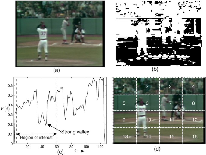

  

  Pitching scene detection. (a) a sample pitching scene, (b) detected field pixels (shown in black), (c) vertical profile V(i) of the field pixels, and (d) 16 blocks dividing the image.

• ii) Layout condition ( C _L ): In pitching scenes, the lower half of the image usually contains more baseball field pixels [36]. Thus, if the lower half has more than twice the number of field pixels compared to the upper half, we set C _L =1, else 0, which becomes:

  if

  $$\sum _{i=1}^W\sum _{j=1}^{H/2}{I}_f(i,j)\ge 2\sum _{i=1}^W\sum _{j=H/2+1}^H{I}_f(i,j)$$

  then C _L =1, otherwise C _L =0.

• iii) Vertical profile condition ( C _V ): The vertical distribution of the field pixels V(i) is given by the equation

  $$V(i)=\frac{1}{H}\sum _{i=1}^H{I}_f(i,j).$$

  (11)

  In pitching scenes, a strong valley is usually found in the left hand side of this distribution [36], as shown in Figure 12c, due to the presence of the pitcher. If such a valley is found, C _V =1; else 0.

• iv) Player location condition ( C _P ): From the video frame, a binary edge image is calculated using the ‘sobel’ method and image dilation [37] is performed. The resulting image is then divided into 16 equal blocks as shown in Figure 12d. In pitching scenes, a higher intensity in the edge-dilated image will be observed in blocks 7, 10, 11, and 14 due to the presence of the pitcher and the batter [8]. If the image intensity of these regions is greater than the average intensity of the image, C _P =1; else 0.

From our observations, almost all pitching scenes fulfill the condition C _V , but not C _A . Thus, unlike in [15], we declare the i th frame as a pitching scene if the following expression yields TRUE:

$$C_{\text{pitch}}=C_V·(C_L+C_A+C_P).$$

(12)

Here, + and · indicate the boolean OR and AND operations, respectively. In [15], we assumed that all pitching scenes satisfy C _A and are used as an AND condition in C _pitch. Using the proposed logic, we successfully detect the pitching shots with an 80.6% accuracy for the baseball games under consideration.

4.2 Audio processing

4.2.1 Speech/non-speech classification

We use an unsupervised non-stationarity measure-based speech /non-speech classification scheme as presented in [15]. The approach is based on a long-term standard deviation calculated on the Mel-filter bank energies (MFBE) of the audio frames, which is sensitive to non-stationarity, and found to be efficient at distinguishing audio environments. If m _{i j} indicates the Mel-filter bank energy of the j th audio-frame and i th filter-bank, we use 40 filter banks (i.e., i=1,…,40) where each audio frame is 25-ms long with a 10-ms overlap, then signal non-stationarity is estimated by computing the standard deviation of MFBE over a longer time-period termed as segments. Here, σ _{k j} will be the k th standard deviation for the j th Mel-filter which is denoted by:

$${\sigma }_{\mathit{\text{kj}}}=\sqrt{\frac{1}{N_s}\sum _{i=(k-1)N_s+1}^{k{N}_s}{\left(m_{\mathit{\text{ij}}}-\frac{1}{N_s}\sum _{i=(k-1)N_s+1}^{k{N}_s}{m}_{\mathit{\text{ij}}}\right)}^2},$$

(13)

where N _s is the number of frames in the time period. In this study, N _s =20 is used (e.g., 200 ms total duration window). Next, we form a vector, σ _k =(σ _{k 1},σ _{k 2},…,σ _kM ), (M=40). The standard deviation of the components σ _k given by s t d(σ _k ) is found to be efficient at distinguishing audio environments. Using this measure, speech/background classification was performed on the game audio using a two mixture GMM as discussed in [15]. Figure 13 shows the probability distribution of s t d(σ _k ) for speech and compares it to different acoustic environments such as outdoors (walking between different locations on campus), cafeteria (fully occupied during lunch hours), and computer cluster room (room consists of multiple servers). The distributions reveal that speech and background are easily separable within the feature space. Thus, a simple unsupervised segmentation algorithm that uses the proposed non-stationarity measure is presented. In the implementation, s t d(σ _k ) is computed for each segment of the game video and a two-mixture GMM is trained using the non-stationarity measure utilizing the expectation-maximization (EM) algorithm. The underlying intuition exploited here is that one Gaussian would learn speech, while the other is expected to learn the background distribution characteristics. This learning is exploited by computing the posterior of each mixture component for every feature P _g (k) as

$$P_g(k)=\frac{1}{\sqrt{2\pi }{\sigma }_g}exp\left[\frac{{(\mathit{\text{std}}({\sigma }_k)-{\mu }_g)}^2}{2\underset{g}{\overset{2}{\sigma }}}\right],$$

(14)

Figure 13

Feature distribution for various acoustic environments.

where μ _g and ${\sigma }_g^2$ are the mean and variance of the g th Gaussian (g=1,2). Using the P _g (k) values, each segment is assigned to the more likely Gaussian (i.e., the one with the higher posterior probability). Since the non-stationarity of speech is typically higher than that of the background, the Gaussian with the larger mean is assumed to be speech. Using this intuition, speech and background Gaussians within the GMM are identified and every k th segment is assigned to either speech or background. Furthermore, Viterbi smoothing is used to smooth the above decisions using a high self-transition probability (0.9∼0.99). This segmentation is used for our speech excitement level detection scheme. Using the above technique on audio data from the six baseball games (about 15 h of audio), an overall accuracy of 80.1% is obtained with a low miss rate of 2.6% (miss is speech detected as background) and false alarm rate of 17.3% (false alarm here represents the background detected as speech).

4.2.2 Excitement measurement in speech

Using the features discussed in section 3, a GMM-based classifier is designed to detect high and moderate excitement levels from the game audio. Details of the evaluation of this scheme is presented later in section 5.1 within other evaluations from this study. This section describes how the excitement classification output is used in construction of the feature parameter for highlights extraction.

To estimate the required G _i (t) functions for high and moderate/low excitement in speech, we use the same principle used for slow motion feature. First, we form the function Φ ₄(t), such that Φ ₄(t)=1 if the high excitement class was detected at time instant t, and 0, otherwise. Similarly, we form Φ ₅(t) for the detected moderate/low excitement class. Time domain examples of these functions are shown in Figure 13d,e. Next, the corresponding G _i (t) functions are computed following Equation 8. The only difference here is that the function Φ ₅(t) is inverted before filtering, following the fact that low excitement in speech is inversely proportional to the viewer arousal.

4.2.3 Audio energy measure

To compute the audio energy, a fixed audio segment size of 267 samples is chosen to be equivalent to our video frame rate of 29.97 frames/section. For each frame t, the audio energy Φ ₆(t) is extracted and later filtered using Equation 8 to obtain G ₆(t). Finally, the averaged value of G ₆(t) in the k th segment is used to compute the segmental audio energy features x _i (k).

4.3 Feature fusion and highlights generation

In order to generate the highlights time curve H _M (t) [10], the functions G _i (t) are filtered using a weighting function,

$$w(t)=\frac{1}{2}\left(1+\text{erf}\left(\frac{{\bar{G}}_M(t)-d}{\sigma }\right)\right)$$

(15)

to obtain,

$$G_i^{\prime }(t)=G_i(t)w(t),\text{with}i=1,\dots ,D$$

(16)

where D=6 is the number of features, and the choice of d=40 and σ=5 follows [10], and

$${\bar{G}}_M(t)=\underset{i}{min}\left[{\text{sort}}_i^M(\{G_i(t)|i=1\cdots D\})\right].$$

(17)

Here, sort${}_i^M$ provides the top M values of G _i (t) at time location t. We use M=3 here. Finally, the highlights time curve is generated as,

$$H_M(t)=\left[\frac{\underset{t}{max}(a(t))}{\underset{t}{max}(ã(t)}\right]ã(t),$$

(18)

where

$$\begin{array}{l}a(t)=\sum _i{\eta }_i{G}^{\prime }(t),\\ ã(t)=K_t(l,\beta )\ast a(t),\text{and}\\ \sum _i{\eta }_i=1.\end{array}$$

To estimate excitability in segment k, we use the averaged values of H _M (t) in that segment to obtain ${\bar{H}}_M(k)$.

For the proposed excitability measure, first, the multi-modal feature vector x(k)=(x ₁(k),x ₂(k)⋯x _D (k)) is computed for each segment k. All features are normalized to zero mean with unit variance before further processing. Next, the histogram of the x _i (k) values across all segments of the video is used to estimate the PDFs $f_{X_i}(\lambda )$. The excitability measure ζ(k) from each segment can then be computed using Equation 3. Note that in this implementation, ζ(k) measure is calculated without a need of any prior knowledge about the features x _i (k). In order to generate a highlight video, segmentation is performed using the detected pitching shot locations. The proposed measure is then used to rank order and combine the video segments according to the user-defined overall highlights duration. Sample highlights generated using the proposed technique can be found in http://sites.google.com/site/baseballhighlights/.

4.4 Generation of excitement time curve

In many applications, a continuous estimate of the excitement level is desired. The proposed technique can also be used to generate such a curve. In this case, the method is directly applied on G _i (t) functions instead of the segmental feature parameters x _i (k). The pitching shot detection is no longer required for this analysis. A sample of such a highlights curve extracted from a baseball video segment of about 20 min is shown in Figure 14. The excitement time curve H _M (k) extracted following [10] is also shown for comparison. We note that the ground truth/real user excitement curve was not estimated for comparison. The plot in Figure 14 is simply a demonstration of the proposed method’s ability to generate a continuous curve as in [10], as well as evaluating the excitement of a video segment.

Figure 14

Excitement time curve generated from a baseball game segment as in [CR10] ( H _M (k) ) and using proposed surprisal measure ( ζ(k) ).

4.5 Real-time implementation

In real-time highlight generation, important highlight events (e.g., a home run or a goal, etc.) are detected and played back immediately or sent to the users through online media. These methods usually work on explicitly detecting the important events using game dependent cues. Since the proposed scheme functions on low-level features and estimates excitability using a probabilistic measure, real-time event detection and broadcast is not feasible in the current framework. However, the method can be extended to operate in real-time by processing video segments in chunks and updating the highlights periodically. Though on-line highlight generation is not the focus of this study, we describe here how this can be achieved using the proposed framework.

In this scenario, the excitability measure ζ(k) requires to be estimated in real-time from the past N segments as

$$\zeta (k)=-{log}_2\prod _{i=1}^D{\int }_{x_i(k)}^{\infty }{\widehat{f}}_{X_i}(\lambda )\mathrm{d}\lambda ,$$

(19)

where ${\widehat{f}}_{X_i}$ indicates the PDF estimate of the i th feature at segment k obtained from the past M segments. The PDFs may also be estimated from all the video segments starting from the beginning of the game up to segment k. For finding a highlight event within the last M segments, a predefined threshold τ on ζ(k) can be used. This threshold can be estimated from the ζ(k) values from the past M segments. This means that if the excitability measure found in the current segment k is significantly high compared to what was observed in the past M segments, segment k is used as highlight. This approach is summarized in Algorithm 1. It should be noted that, after the game is over, the highlights generated form the full video may not contain all the local ‘short-time’ highlight segments that were detected in real-time.

Algorithm 1 Real-time highlight generation using the proposed framework

5 Evaluation of proposed system

In this section, we first evaluate the speech production-based classifier in terms of the excitability measure for sports commentators speech. Next, we perform a subjective evaluation of the complete audio-video highlights extraction system combining the multi-modal features.

5.1 Speech production-based classifier

As discussed in section 3, fundamental frequency F ₀, spectral center of gravity SCG, and the first three formants F ₁₋₃ were found to provide good correlation with the perceptual excitement labels and hence are used in this section as input parameters for automatic excitement-level assessment.

The speech-based classifier utilized in the curently proposed highlights generation scheme replicates the one presented in our preliminary study [15]. Two GMMs are trained to represent ‘moderate’ excitement (referring to excitement levels 1 and 2) and ‘high’ excitement (levels 3 and 4). The 32-mixture GMMs are trained on samples extracted from 4 baseball games, where the subjective excitement-level labels serve as target transcriptions of the data, and evaluated on 2 remaining games representing the open test set. The binary classification results are evaluated by means of equal error rate (EER). In a round robin experiment, the classifier utilizing features normalized by the game level statistics provides EER of 21.4 to 22.4 %, see [15] for details.

The feature normalization utilized in the previous paragraph assumes that the whole game is available to estimate the global statistics of the commentator’s speech (see section 3). Some applications may require generation of highlight previews while the game is still in progress. In such a case, the statistics of commentator’s speech features may be estimated on-the-fly. One possible approach is to estimate the feature means and standard deviations from the starting segment of the game and cumulatively update their values with every newly observed speech island. It is expected that the cumulative statistic estimates will converge over time towards the global game statistics.

To evaluate how the on-the-fly estimation might impact the accuracy of the excitement level classification, we implement a simple scheme where the statistics estimated from the initial segment of the game are continuously updated based on the newly observed speech islands using a weighted mean. The currently available estimates are used to normalize features extracted from the current voiced island. Clearly, there would be an option to go back in time and re-normalize all past segments with the newest estimates; however, we do not utilize this option in our current study.

The speech-based excitement level classification results for the on-the-fly approach are summarized in Figures 15 and 16. The first figure compares average game EERs for classifiers utilizing on-the-fly feature normalization (initial estimation segments of lengths 50 and 3,000 s) and a classifier employing game level statistics (‘Whole Game’). The EERs are averaged across three round robin experiments and the vertical bars represent their standard deviations. It can be seen that there is a benefit from using game level statistics but the performance drop when switching to on-the-fly processing with an initial segment of 50 s is quite affordable (approximately 1.4 % absolute EER increase).

Figure 15

Impact of on-the-fly estimation of commentator’s speech statistics on excitement level classification error. Game level equal error rates for initial estimation segments of different lengths.

Figure 16

Impact of on-the-fly estimation of commentator’s speech statistics on excitement level classification error. Equal error rate as a function of initial estimation segment length and game time.

Figure 16 details the averaged round robin EERs as functions of the elapsed game time. A 1-min-long window was applied to smooth the temporal EERs. It can be seen that the classifier utilizing game level statistics performs more accurately through a major part of the game; however, besides the first 4 min of the game, where the EER difference for both 50- and 3,000-s setups versus the game level setup drops by nearly 9 % EER, the EER difference for the global and on-the-fly systems does not exceed more than approximately 3 %, which seems quite affordable.

5.2 Subjective evaluation of the highlight generation system

In order to evaluate the effectiveness of the proposed measure of excitability, we conducted an independent subjective evaluation involving five viewers familiar with the game of baseball. We note that subjective evaluation of video summarization is quite challenging since it requires each subject to watch the entire game (typically approximately 3-h long), memorize all exciting moments and then select the most exciting parts to assess if the algorithm properly selected the highlights. In addition, it is natural to have a strong disagreement between viewers in deciding which scene should be selected/rejected. To make the evaluation feasible, we selected 100 pitching scenes (semantic segments) of about 15 s in duration from a baseball game. The subjects were asked to watch the videos and rank the excitability of the scene on a scale from 0 to 30. The rubrics used are boring (0 to 10), moderately exciting (10 to 20), and very exciting (20 to 30). Since the dynamic range of the ranking scores may vary across subjects, the scores obtained from each subject are normalized to zero mean and unit variance, and then averaged to obtain the final subjective measure. Note that the normalization here does not affect the ranking order of the segments decided by the subject (i.e., order from lowest ranking to highest ranking scenes will be preserved and also segments eligible to form highlights remain the same). Next, we extract excitement estimation in the selected 100 video segments obtained from (i) ${\bar{H}}_M(k)$ computed using [10], (ii) γ(k) computed from a simple addition and normalization of the feature parameters x _i (k) [15], and (iii) the proposed measure ζ(k). The measures are evaluated by comparing their correlation and ranking agreement with the subjective measure.

5.2.1 Correlation between individual features and subjective scores

At first, we analyze how each feature parameter used in this study is correlated to the subjective user excitability. For data points, y _i and z _i , i={1,…,N}, the correlation coefficient ρ is calculated as

$$\rho =\frac{\text{cov}(y,z)}{{\sigma }_y{\sigma }_z}=\frac{{\sum }_{i=1}^N(y_i-\bar{y})(z_i-\bar{z})}{\sqrt{{\sum }_{i=1}^N{(y_i-\bar{y})}^2{\sum }_{i=1}^N{(z_i-\bar{z})}^2}}.$$

(20)

This equation is used for calculating the correlation between the feature coefficients x _i (k) and the subjective scores (ζ(k), γ(k), or ${\bar{H}}_M(k)$). The correlation of the individual features with the subjective scores are summarized in Figure 17 and Table 2. Here, we observe that all of the selected feature parameters x _i (k) are correlated with the subjective scores with positive values (i.e., they are proportional to excitability). Also, in each correlation value in Table 2, the probability of the null hypothesis (p value) is p<0.05 (i.e., the correlation is significant).

Figure 17

Correlation coefficients of different feature parameters/objective excitement measures and subjective evaluation scores. Excitement measures are computed by fusing the feature parameters using equal weights.

Table 2 Comparison of correlation coefficient ( ρ ) between different feature parameters and subjective evaluation scores

Looking closely at Figure 17, we conclude that for our particular case, the most effective feature parameter is the average camera motion, with the highest individual correlation coefficient (ρ=0.6531). This is an indication that camera movement is more prominent during exciting moments of a baseball game, which is probably not the case for tennis, where the camera is more or less stationary. Excitement level detected in commentator speech is another good indication of excitability (ρ=0.5146). This is more or less true for any sports. The slow motion feature is also highly correlated with excitability (ρ=0.5066).

Observing the individual contribution of the features towards the excitability measure, we now like to analyze the effect of different feature weights η _i in (3). We use three different weight vectors η=[η ₁…η _D ]:

• 1. Equal weights: η _i =1/D=1/6. Weight vector: w ₀= [ 1 1 1 1 1 1]/6

• 2. Higher weights to features x ₁(k) & x ₂(k): w ₁= [ 2 2 1 1 1 1]/8

• 3. Higher weights to features x ₂(k) & x ₄(k): w ₂= [ 1 2 1 2 1 1]/8

These weight settings are motivated by the higher correlation these individual features demonstrate (slow motion, high audio excitement and camera motion activity). In practical applications, we will not be able to estimate the correlation values since the subjective scores will not be available. However, using a development dataset, these weights can be trained and later applied during evaluation.

5.2.2 Correlation between subjective and objective scores

When equal weights are used for the parameters η _i in (3), the proposed excitability measure ζ(k) is seen to have the highest correlation coefficient of 0.77473, which outperforms the other two excitability measures γ(k) and ${\bar{H}}_M(k)$, yielding correlations of 0.67579 and 0.59287, respectively. This indicates the effectiveness of the proposed measure in fusing multiple feature parameters. These values are also shown in Figure 17, indicating that the subjective scores are better correlated with the proposed excitability measure, as opposed to the individual features.

Similar to the previous section, we compute these correlation coefficients for the alternative feature weights w ₁ and w ₂. The results are summarized in Table 3, columns 6 and 7. With the weight setting of w ₁, the proposed method provides a correlation value of 0.80145, which is again superior compared to the other methods shown. The corresponding p values here again verify that the correlation values are significant (p<0.05).

Table 3 Performance evaluation by comparing top N highlight segments selected using subjective and objective methods

5.2.3 Comparison between subjective and objective highlight rank

To evaluate objective rank ordering of the segments, we choose N top subjectively ranked video segments as a ground truth for highlights. We use the following values: N={10,20,30,40}. The excitement ranking measures ${\bar{H}}_M(k)$, γ(k), and ζ(k) are then evaluated with respect to accuracy, true-positive rate (TPR) and false positive rate (FPR). For equal feature weights, the results are summarized in Figure 18. Here, again, we observe that the proposed measure provides superior performance compared to [10] and [15] for most values of N. For the alternative feature weights w ₁ and w ₂, the TPR values for different N s are summarized in Table 3, columns 2 to 5. In each of these cases, we find that the proposed method provides superior performance (in italics).

Figure 18

Performance evaluation by comparing top N highlight segments selected using subjective and objective measures. Accuracy(%) and true-positive and false-positive rates are shown. In the plot, ${\bar{H}}_M(k)$, γ(k), and ζ(k) indicate the methods in [10][15], and the proposed one.

As an example, for N=20, the proposed technique selects 70% of the top 20 subjectively ranked segments with an FPR of 7.5%, while for [10], the TPR and FPR values are 55% and 11.2%, respectively. With proper design of the feature weights, the highlight selection performance can improve further as shown in Table 2.

6 Conclusion

A generic video highlights generation scheme based on an information theoretic measure of user excitability was presented. The scheme utilizes audio excitement and low-level video features. Based on the analysis of the sports commentator’s speech, production parameters most correlated with the perceptual excitability were selected to form an acoustic feature vector for excitement assessment. Along with this, audio energy, slow motion duration, camera motion, and scene-cut density were used as features in the highlights extraction system. The proposed integrated excitability measure was shown to effectively combine the multi-modal features in video segments and found to be highly correlated with a perceptual assessment of excitability. The proposed scheme was also shown to outperform state-of-the-art generic excitability ranking methods.

Endnote

^a Outcomes of this study were presented in short forms in our preliminary studies [15, 16].

Example Processed Output Content

The following websites provide sample processed output time domain highlight compressed video content using the CRSS-UTDallas proposed system developed in this study.

http://sites.google.com/site/baseballhighlights/

http://crss.utdallas.edu/demos/

References

Pan H, Van Beek P, Sezan M: Detection of slow-motion replay segments in sports video for highlights generation. Proc. IEEE ICASSP 7–11 May 2001
Delakis M, Gravier G, Gros P: Audiovisual integration with Segment Models for tennis video parsing. Comput. Vis. Image Underst 2008, 111(2):142-154. 10.1016/j.cviu.2007.09.002
Fleischman M, Roy B, Roy D: Temporal feature induction for Baseball highlight classification. In Proceedings of the 15th Int. Conf. on Multimedia, Augsburg, Germany, 24–29 Sept.. New York: ACM; 2007:333-336.
Xiong Z, Radhakrishnan R, Divakaran A: Generation of sports highlights using motion activity in combination with a common audio feature extraction framework. Proc. IEEE ICIP, Barcelona, Catalonia, 14-17 Sept. 2003.
Kolekar M, Sengupta S: Semantic concept mining in cricket videos for automated highlight generation. Multimedia Tools and Appl 2010, 47(3):545-579. 10.1007/s11042-009-0337-1
Tjondronegoro D, Tao X, Sasongko J, Lau C: Multi-modal summarization of key events and top players in sports tournament videos. In 2011 IEEE Workshop on Applications of Computer Vision (WACV), Kona, HI, 5–7 January. Piscataway: IEEE; 2011:471-478.
Cheng C, Hsu C: Fusion of audio and motion information on HMM-based highlight extraction for baseball games. IEEE Trans. Multimedia 2006, 8(3):585-599.
Lien C, Chiang C, Lee C: Scene-based event detection for baseball videos. J. of Visual Comm. and Image Representation 2007, 18: 1-14. 10.1016/j.jvcir.2006.09.002
Assfalg J, Bertini M, Bimbo AD, Nunziati W, Pala P: Soccer highlights detection and recognition using HMMs. In Proc. ICME ’02, Lausanne, Switzerland, 26-29 Aug. 2002 Volume 1. Piscataway: IEEE; 2002:825-828.
Hanjalic A: Adaptive extraction of highlights from a sport video based on excitement modeling. IEEE Trans. Multimedia 2005, 7(6):1114-1122.
Xiong Z, Radhakrishnan R, Divakaran A, Huang T: Audio events detection based highlights extraction from baseball, golf and soccer games in a unified framework. In Proc. IEEE ICASSP, Hong Kong, China, 6–10 April 2003 Volume 5. Washington, DC: IEEE Computer Society; 2003:632-635.
Chang P, Han M, Gong Y: Extract highlights from baseball game video with hidden Markov models. In Proc. Image Process., Rochester, New York, 22–25, Sept. Volume 1. Piscataway: IEEE; 2002:609-612.
Rui Y, Gupta A, Acero A: Automatically extracting highlights for TV baseball programs. In Proceedings of the Eighth ACM International Conference on Multimedia, Los Angeles, CA, October 30 – November 03. New York: ACM; 2000:115-115.
Ma Y, Lu L, Zhang H, Li M: A user attention model for video summarization. In Proceedings of the tenth ACM international conference on Multimedia, Juan les Pins, France, 1–6 December, 2002. New York: ACM; 2002:542-542.
Bořil H, Sangwan A, Hasan T, Hansen JHL: Automatic excitement-level detection for sports highlights generation. Proc. InterSpeech, Makuhari, Chiba, Japan 26–30 September 2010 2202-2205.
Hasan T, Bořil H, Sangwan A, Hansen JHL: A multi-modal highlight extraction scheme for sports videos using an information-theoretic excitability measure. IEEE ICASSP, Kyoto, Japan 25–30, March 2012 2381-2384.
Cover TM, Thomas JA: Elements of Information Theory. New York: Wiley-Interscience; 1991.
Hansen JHL: Analysis and compensation of speech under stress and noise for environmental robustness in speech recognition. Speech Comm 1996, 20(1-2):151-173. 10.1016/S0167-6393(96)00050-7
Cowie R, Cowie Douglas-E, Tsapatsoulis N, Votsis G, Kollias S, Fellenz W, Taylor JG: Emotion recognition in human-computer interaction. IEEE Signal Process. Mag 2001, 18: 32-80. 10.1109/79.911197
Bořil H, Kleinschmidt T, Boyraz P, Hansen JHL: Impact of cognitive load and frustration on drivers’ speech. The J. Acoust. Soc. Am 2010, 127(3):1996-1996.
Lee CM, Narayanan SS: Toward detecting emotions in spoken dialogs. IEEE Trans. on Speech & Audio Process 2005, 13(2):293-303.
Sjolander K, Beskow J: Wave Surfer-an open source speech tool. Proc. of ICSLP‘00, Beijing, China, 16–20 Oct. 2000 Volume 4
Schulman R: Dynamic and perceptual constraints of loud speech. The J. Acoust. Soc. Am 1985, 78(S1):S37-S37.
Gramming P, Sundberg S, Ternström S, Perkins W: Relationship between changes in voice pitch and loudness. STL-QPSR 1987, 28: 39-55.
Lu Y, Cooke M: Speech production modifications produced by competing talkers, babble, and stationary noise. The J. Acoust. Soc. Am 2008, 124(5):3261-3275. 10.1121/1.2990705
Pisoni D, Bernacki R, Nusbaum H, Yuchtman M: Some acoustic-phonetic correlates of speech produced in noise. In Proc. of ICASSP, Tampa, Florida, 26–29 March, Volume 10. Piscataway: IEEE; 1985:1581-1584.
Kent RD, Read C, San Diego: The Acoustic Analysis of Speech. Whurr Publishers; 1992.
Bond Z, Moore T: A note on Loud and Lombard speech. Proc. of ICSLP‘90, Kobe, Japan, 18–22 November 1990
Bořil H: Robust speech recognition: analysis and equalization of Lombard effect in Czech Corpora, PhD thesis. Czech Republic: Czech Technical University in Prague; 2008. http://www.utdallas.edu/~hxb076000
Junqua JC: The Lombard reflex and its role on human listeners and automatic speech recognizers. The J. Acoust. Soc. Am 1993, 93: 510-524. 10.1121/1.405631
Wakita H: Normalization of vowels by vocal-tract length and its application to vowel identification. IEEE Trans. Acoust. Speech and Signal Processing 1977, 25(2):183-192. 10.1109/TASSP.1977.1162929
Oppenheim A, Schafer R: Discrete-Time Signal Processing. Upper Saddle River, NJ: Prentice Hall; 1999.
Liu C, Huang Q, Jiang S, Xing L, Ye Q, Gao W: A framework for flexible summarization of racquet sports video using multiple modalities. Comput. Vis. Image Underst 2009, 113: 415-424. 10.1016/j.cviu.2008.08.002
Liu H, Zhang Wj, Cai J: A fast block-matching algorithm based on variable shape search. J. Zhejiang University - Science A 7: 2006. [10.1631/jzus.2006.A0194]
Truong B, Dorai C, Venkatesh S: New enhancements to cut, fade, and dissolve detection processes in video segmentation. In Proc. of the 8th ACM Inter. Conf. on Multimedia, Los Angeles, CA, October 30 – November 03, 200. New York: ACM; 2000:227-227.
Chu W, Wu J: Explicit semantic events detection and development of realistic applications for broadcasting baseball videos. Multimedia Tools and Appl 2008, 38: 27-50. 10.1007/s11042-007-0145-4
Van Den Boomgaard R, Van Balen R: Methods for fast morphological image transforms using bitmapped binary images. Graphical Models and Image Process 1992, 54(3):252-258.
Acknowledgements
This project was funded by the AFRL under contract FA8750-12-1-0188 (Approved for public release, distribution unlimited), and partially by the University of Texas at Dallas from the Distinguished University Chair in Telecommunications Engineering held by J.H.L. Hansen.
Author information
Authors and Affiliations
Corresponding author
Additional information
Competing interests
The authors declare that they have no competing interests.
Authors’ original submitted files for images
Below are the links to the authors’ original submitted files for images.
Rights and permissions
Open Access This article is distributed under the terms of the Creative Commons Attribution 2.0 International License ( https://creativecommons.org/licenses/by/2.0 ), which permits unrestricted use, distribution, and reproduction in any medium, provided the original work is properly cited.
About this article
Cite this article
Hasan, T., Bořil, H., Sangwan, A. et al. Multi-modal highlight generation for sports videos using an information-theoretic excitability measure. EURASIP J. Adv. Signal Process. 2013, 173 (2013). https://doi.org/10.1186/1687-6180-2013-173
Received:
Accepted:
Published:
DOI: https://doi.org/10.1186/1687-6180-2013-173