- Research
- Open access
- Published:
Analysis of frequency domain frame detection and synchronization in OQAM-OFDM systems
EURASIP Journal on Advances in Signal Processing volume 2014, Article number: 83 (2014)
Abstract
For future communication systems, filter bank multicarrier schemes offer the flexibility to increase spectrum utilization in heterogeneous wireless environments by good separation of signals in the frequency domain. To fully exploit this property for frame detection and synchronization, the advantage of the filter bank should be taken at the receiver side. In this work, the concept of frequency domain processing for frame detection and synchronization is analyzed and a suitable preamble design as well as corresponding estimation algorithms is discussed. The theoretical performance of the detection and estimation schemes is derived and compared with simulation-based assessments. The results show that, even though the frequency domain algorithms are sensitive to carrier frequency offsets, satisfactory frame detection and synchronization can be achieved in the frequency domain. In comparison to time domain synchronization methods, the computational complexity increases; however, enhanced robustness in shared spectrum access scenarios is gained in case the described frequency domain approach is utilized.
1 Introduction
The increasing practical interest in filter bank multicarrier systems for next-generation wireless communication systems raises the demand for efficient synchronization methods making use of the favorable frequency containment of the filter bank to improve robustness in spectrum sharing scenarios. The focus of this work is on offset quadrature amplitude modulation orthogonal frequency division multiplexing (OQAM-OFDM), since this modulation scheme provides optimal bandwidth efficiency with respect to symbol density in the time-frequency grid [1]. Common data-aided synchronization schemes, e.g., [2], use the time domain signal for symbol timing offset (STO) and carrier frequency offset (CFO) estimation. In this case, the analysis filter bank at the receiver is not involved and the advantage of separation of subchannels offered by the filter bank multicarrier systems is disregarded. As a result, the time domain synchronization in spectrum sharing scenarios needs to be enhanced, for example, by introducing a prefiltering stage, and its complexity increases.
In [3], Stitz et al. make use of the analysis filter bank for synchronization and propose a method based on a training sequence embedded into each subchannel that enables a per-subchannel evaluation of the received signal. The authors showed that the interference from neighboring subchannels limits the estimation range of the CFO. The task of STO correction is thereby left to a three-tap equalizer, which lowers the demand for accurate STO estimation. For that reason, only frame detection is considered. The same authors describe a pilot-based approach for frequency domain synchronization in [4], proposing a closed-form approach to STO and CFO estimation. The training sequence is embedded as pilots in the payload data, which results in a limited detection range when the STO and CFO are estimated directly. In [5], Saeedi-Sourck and Sadri utilize a modified preamble structure, which has been originally proposed in [6], and that mitigates the effect of self-interference by occupying only every second subchannel. Closed-form CFO estimation is enabled by the repetition of identical preamble symbols. The STO is estimated based on the received energy in the frequency domain as also mentioned in [6]. The STO estimation demands for a sample-wise demodulation of the received preamble as well as for a sufficiently large gap between preamble and payload to find the maximum of the metric. Based on a reduced version of this preamble, the same authors propose an iterative approach to CFO and STO estimation in [7] that comes close to the maximum likelihood estimator. Both contributions, however, face the drawback of sample-wise demodulation that leads to a high complexity, for which reason they are not considered for comparison in this work. In [8], we proposed a synchronization scheme that utilizes a similar approach to preamble design compared with that of Saeedi-Sourck and Sadri in [5] to minimize the effects of interference, yet only symbol-wise demodulation of the received signal is necessary for CFO and STO estimation. This leads to a reduced complexity compared to sample-wise processing. Additionally, our design reduces the gap of unused symbols between preamble and payload by utilizing auxiliary pilots to remove self-interference [4]. It enables the estimation of offsets in a range that is comparable to common time domain synchronization methods while keeping the amount of training sequence overhead small.
In this work, the performance of the frame detection algorithm and the Cramér-Rao vector bound (CRVB) of the STO and CFO estimation are derived analytically based on the proposed training sequence structure from [8]. The performance of the proposed STO and CFO estimation algorithms is evaluated against the CRVB followed by the assessment of two different synchronization concepts. The proposed concepts show an improved estimation range compared to previously known frequency domain methods and achieve a performance that is similar to the one of commonly used time domain solutions. The focus of this analysis is on preamble-based direct estimation algorithms due to their reasonable trade-off between efficiency and complexity. For that reason, interference cancelation techniques are not considered.
The paper is structured as follows. In Section 2, the signal model including the preamble design is specified. The detection and estimation metrics are introduced in Section 3, followed by the analytical derivation of their performance. Section 4 shows and discusses the results. The conclusion from this work is provided in Section 5.
2 System model and preamble design
In OQAM-OFDM, the real and imaginary parts of the complex-valued QAM modulated symbols are staggered in time by half a symbol period T/2. The resulting real-valued symbols dk,m are multiplied by the factor θk,m=jmod(m+k,2), depending on the symbol index m and subchannel index k, enabling the real-field orthogonality of the OQAM-OFDM symbols.
Modulation of the symbols dk,m with the synthesis filter bank results in the time-discrete output signal
with the sample rate of . k is chosen from the set of available subchannels , and T=K T s is the symbol duration with K equal to the overall number of subchannels. p[n T s ] is the time-discrete prototype filter function of length β T with β representing the overlapping factor of the time domain symbols. It is beneficial to use well-localized pulse shapes in both time and frequency domains to reduce the effect of self-interference due to synchronization errors, to improve performance in doubly dispersive channels, and to lower out-of-band emissions [1]. It is assumed here that the filters’ transfer function only overlaps with the adjacent subchannels. For a detailed analysis of the OQAM-OFDM scheme and its properties, the reader is referred to [9]. The received signal r[n T s ], which contains the zero-mean circular-symmetric Gaussian noise η[n T s ], can be described as
The STO τ is defined in integer values of T s , and the CFO ν is normalized with respect to the subchannel spacing 1/T. A common phase shift is described by ϕ. For the following analytical derivation, the channel impulse response h[n T s ] is neglected. Passing the received signal through the analysis filter bank yields the unsynchronized demodulated symbols
with the filtered noise samples Ψk,m.
One of the critical issues related to frequency domain processing is the mismatch between synthesis and analysis filter bank in the case of STO and CFO. The degradation of the received amplitude of the signal and the introduction of interference from neighboring symbols put limits on the performance of the frequency domain processing [4]. By separation of the pilots in time and frequency direction within the preamble, the self-interference is reduced.
The preamble design that is utilized here has first been presented in [8] and provides a trade-off between low self-interference and an appropriate offset estimation range for both STO and CFO. The preamble occupies every second subchannel only and every second OQAM-OFDM symbol for separation of the pilots. The pilot spacing in time and frequency direction allows the STO and the normalized CFO to be estimated in the range of {−T/4+T s ,⋯,T/4−T s } and (−0.5,0.5), respectively. An example of the structure of a frame using the described training sequence is given in Figure 1. A preamble design based on a similar structure has been proposed for synchronization in [5] where the preamble and the payload part are completely separated by guard symbols to lower the interference which results in additional overhead of the training sequence. In our proposed preamble, auxiliary pilots, described in [10], can mitigate the distortion of the preamble symbols caused by the succeeding payload symbols, facilitated by subtracting the pre-known interference from the preamble symbols.

Representation of the frame structure. Frame in the subchannel-symbol grid including the pilots, the auxiliary pilots, and the payload data symbols.
This interference from the surrounding payload symbols is obtained prior to transmission with the help of the distortion-free system response of the synthesis and analysis filter banks. Their use reduces the amount of guard symbols needed between preamble and payload part to a minimum while limiting the interference from the payload part. It is worth to note here that sparsely occupied preambles are also used for channel estimation for similar reasons, as discussed in [11].
For the analytical treatment, the auxiliary pilots and the payload part are not taken into account. The preamble is defined as
with λ k ∈{−1,1}. The subset of only contains K2=K u /2 subchannels with either even- or odd-numbered indices out of the set of utilized subchannels . K u is equal to the number of subchannels used for transmission. The sequence bk,m can be arbitrarily chosen and optimized, e.g., to achieve a low peak-to-average power ratio.
For the pilots in the preamble, we assume a pilot boost factor of , resulting in dk,m=γ bk,m and . As a result from the sparse preamble design, the factor θk,m is the same for each pilot symbol. Hence, without loss of generality, the factor θ is assumed to be 1 and neglected in the following. Given this, (1) and (3) lead to the signal model of the preamble, which is used in the following for the analytical derivation of the CRVB. describes the recovered but not synchronized preamble pilots at the receiver after the demodulation.
As a result from the design of the prototype filter function in OQAM-OFDM and the preamble structure in Figure 1, the frequency domain samples can be considered mutually separated. For that case Ψk,m has the same statistical properties as η[n T s ] as derived in Appendix 1 from (3).
is obtained for m=0 and
for m=2. can be rewritten more compactly as
a0(τ,ν) and a2(τ,ν) are functions of τ and ν and correspond to the ambiguity functions of the prototype filter function p[n T s ]. Furthermore, a0(τ,ν) and a2(τ,ν) only differ in phase, and a(τ,ν)=|a0(τ,ν)|=|a2(τ,ν)| holds. In the following, the parameters τ and ν are neglected for readability. Reformulation of (5) and (7) in matrix notation yields
with
where W=2K2 is the number of demodulated preamble symbols, called observations in the following, that are taken into account. In this notation, each row of a vector or matrix is related to one subchannel, denoted by the index k. In (10), this index directly affects the value of the diagonal elements of the matrix E. Furthermore, the definitions and are used.
3 Detection and estimation
In this section, the metric for frame detection in the frequency domain is introduced and analytically evaluated. Furthermore, the maximum likelihood estimator (MLE) for the CFO is presented and the MLE for the STO is derived. The maximum likelihood estimation of the symbol timing leads to an estimator with an insufficient estimation range for which reason two alternative STO estimators are motivated and described. In addition, the CRVB is obtained as a lower bound on the variance of the estimators.
In time domain processing, the common metric is based on an auto-correlation window that is shifted sample-wise. In frequency domain processing, a sample-wise shift of the received signal requires a complete demodulation process per sample shift, leading to a high complexity. The focus of this work is on symbol-wise demodulation to efficiently perform detection and estimation in the frequency domain. Therefore, the processing is based on the offset-afflicted received pilots obtained after demodulation.
3.1 Frame detection
The preamble needs to be detected in the stream of received symbols before estimation of the STO and CFO. For the decision, the metric to acquire the preamble signal is, as introduced in [12],
Thereby, the superscript.A indicates that the absolute value is taken. The power normalization is approximated by
The index m is discarded in the following for readability. The decision whether a preamble has been acquired or not is performed on the rule
where 0<ρ<1 defines the threshold value. It follows that the detected symbol index is equal to m, if (15) is true. Two measures are of importance to characterize the quality of the detection algorithm: probability of missed detection Pmd and probability of false alarm Pfa. Both probabilities depend on the decision threshold ρ. The first one indicates the probability of a detection failure if a preamble is present but is not detected. The second one provides the probability that a preamble is detected if only noise is received.
We now focus on deriving a suitable threshold value to achieve a desired Pmd, depending on the parameters signal-to-noise ratio (SNR) and the number of observations W. The conditional probability that is below the specific value ρ Q b is given by [13]
The detailed derivations of the probability density functions (PDF) and f(Q b ), and the conditional PDF are given in Appendix 2. Integration over Q b provides the Pmd according to [13]
The Pfa can be derived for the case that only noise is present and holds. Then, the metric C Ψ is defined similar to (13) as
and Q Ψ can be approximated to
A false alarm occurs when the threshold is exceeded, which can be formulated as follows
Here, has been chosen following [13], which allows to simplify the calculation of the PDF. Following the derivation of the PDFs in Appendix 2 and assuming independence of Q Ψ and , the Pfa is given by
For the analytical derivation of the Pfa for the case that payload symbols plus noise are present, the detection metric is performed on the demodulated symbols . However, compared to the case with pure noise, the received symbols are no longer normal distributed but depend on a discrete modulation alphabet. A tractable analytical solution can be obtained only if we approximate the distributions with normal distributions, resulting in expressions for f(Q Ψ ) and that are equivalent to the case of pure noise. Hence, this Pfa case is only evaluated based on simulations in Section 4.
3.2 Frequency offset and symbol timing estimation
After frame acquisition, the symbol index characterizing the start of the preamble sequence is known. As a result, is set to zero in the following. Based on the estimation of the first preamble symbol, a coarse estimation of the CFO, which still suffers from intercarrier and intersymbol interference, can be obtained:
The corresponding metric applied to two identical signal parts in the time domain yields the maximum likelihood estimator for the frequency offset, as derived in [14] and also used in [5]. For small offsets, when the influence of interference and amplitude degradation can be neglected, the metric for the frequency domain yields the MLE for the frequency offset. In case of larger offsets, the estimator is influenced not only by noise but also by interference from neighboring subchannels and the misalignment of the transmit and receive filters. Hence, due to the simplicity and the optimality in case of small offsets, the MLE from [14] is considered a useful and practical solution for frequency domain estimation.
For the estimation of the STO in the frequency domain, the relation
holds with representing the discrete Fourier transform (DFT) operation and the frequency domain samples given by X k . It follows that each received preamble symbol contains information about the parameter τ and that it can be evaluated individually.
The optimal STO estimator is derived from the signal model in (8) as described in the following. The logarithm of the likelihood function l, neglecting irrelevant additive factors, is given by
with the parameter vector v= [τ,ν,ϕ]T, the covariance matrix
and C Ψ being a subset of where only the subchannels with indices are captured, as reflected by the preamble structure. The definition of is given in Appendix 1. Setting the derivative of (24) with respect to τ equal to zero results in the maximum likelihood condition for the STO estimator. For one received preamble symbol , it follows that
with equal to the upper left or lower right submatrix of E, depending on the index i. The last step of calculation is valid under the assumption of small time and frequency offsets, i.e., a i =1. From (26), it follows that the condition for the MLE yields
For ϕ≈0, the simplification sin(x)≈x can be made and the closed-form expression of the MLE yields
Under the assumption that is approximately constant in case of additive white Gaussian noise (AWGN) and for a symmetric allocation of the subchannels, is zero and the MLE becomes independent of the common phase shift ϕ. Merging the estimates results in the MLE
For being a sufficiently large set or at sufficiently high SNR, the MLE is unbiased [15]. The estimation of the MLE is limited by the phase ambiguity of the subchannel with the highest subchannel index k. Setting the maximum subchannel index |k m a x |=K/2−1 into (23) yields the phase of to be smaller than π only for |τ|≤T s . Furthermore, the assumption that ϕ≈0 is not always justified, and therefore, the MLE is not considered a practical option for STO estimation. Nevertheless, the MLE will be used later in Section 4 for verification of the CRVB.
The limitation of the estimation range can be overcome by a suboptimal solution, in which the difference in phase between two neighboring pilots of the same symbol at different subchannels is used. In the following, this method is called closed-form estimator (CFE) and has been proposed for embedded pilot symbols in [4]. The closed-form expression for the estimation of τ is motivated by (23) and formulated as
where Δ k =2 is the difference in subchannel indices of the pilots used in the preamble. The set of available subchannel indices with K p entries is . is a subset of that contains only those indices k where the index k+Δ k is as well an element of . For the estimation to hold, it is assumed that the coherence bandwidth is sufficiently large, such that the pilots at indices k and k+Δ k experience approximately the same phase of the channel [4]. This assumption is not fulfilled in general but is approximately valid as the results in Section 4 confirm. By utilizing a fixed pilot spacing of Δ k =2 as a result of the preamble structure, the STO estimation range is −T/4+T s ≤τ≤T/4−T s . Therefore, the CFE offers a more practical solution compared to the MLE approach. A solution for the condition , which shows that the CFE is unbiased, could not be found in a simple way. For that reason, we focus on the noise-free case only, which allows to illustrate that the estimate is unbiased. By applying on (30), we obtain
Different to this closed-form expression of the STO, the cross-correlation-based estimator (CCE), proposed in [8], is based on finding the which maximizes the absolute value of the cross-correlation . By maximizing this expression, the ML condition in (27) is minimized, which results in the metric
where the estimate of the CFO obtained in (22) is used to counteract the distortion effect of the CFO on the cross-correlation. It is beneficial to choose the set of trial values to be integer values of the sample duration T s , which makes it different from the closed-form estimations, where can result in any real number. Under the assumption that , it is calculated in the following that matches τ for the noise-free case. If irrelevant scaling factors and phase shifts are discarded for simplicity, it follows from (32) that
The expression in (33) is maximized if which indicates that the estimator is unbiased at high SNR.
3.3 Cramér-Rao vector bound
The Cramér-Rao vector bounds for CFO and STO estimation can be derived as a lower bound on the estimation performance of the discussed estimators. The CRVB depends on the parameter vector v=[τ,ν,ϕ]T[15]. The derivation of the regularity condition, as a precondition to the CRVB, is given in Appendix 3. The entries of the Fisher information matrix F are derived, using the the log likelihood function in (24), according to
where for F(i,i) the following identity holds [15]
The derivation of F is provided in Appendix 4. As a0 and a2 are determined by the pulse shape p[n T s ] and are functions of τ and ν, their partial derivatives, and therefore F, have to be evaluated for different pulse shapes individually. Depending on the pulse shape, the derivation of a closed-form expression for the CRVB is difficult to obtain. For that reason, we have opted to use a numerical approach here. The CRVB is then given by the numerical matrix inversion of F according to
Including a Rayleigh fading channel matrix in (8) leads to the same lower bound on the estimation performance as for the AWGN case.
A representation of the analytically derived root mean square error (RMSE) over the offset plane is given in Figures 2 and 3. The pulse shape p[n T s ] is designed following the frequency sampling technique with an overlapping factor β=3 and K=32 and is defined in more detail in Section 4. The RMSE is used as a measure for the accuracy of an estimation. Given that the estimations are unbiased, the CRVB is related to the RMSE according to . In the following, we will focus on the two parameters τ and ν. ϕ, representing the common phase shift, has no effect on the CRVB of τ and ν and is therefore neglected.

RMSE derived from the CRVB for the normalized STO τ/T s plotted over the τ - ν offset plane. SNR = 0 dB.

RMSE derived from the CRVB for the normalized CFO ν plotted over the τ - ν offset plane. SNR = 0 dB. The RMSE of the estimation is strongly influenced by the CFO, while a STO only causes a minor degradation.
4 Results and discussion
In addition to the analytically derived performance of the preamble structure, the core algorithms are evaluated based on simulations. Furthermore, synchronization concepts are assessed by means of the bit error rate (BER). Thereby, the following system parameters and simulation settings are used if not stated otherwise.
-
The number of subchannels K is set to 32 with and . It follows that the number of all usable subchannels is K u =32 and the number of subchannels occupied by the preamble pilots is K2=16. For the simulation results, presented in Figures 4, 5, 6, 7, and 8, the number of payload symbols and auxiliary pilots is set to zero. Otherwise, the number of OQAM-OFDM payload symbols is set to four and 4-QAM modulation is applied. The number of realizations used in simulations is 105.
Figure 4 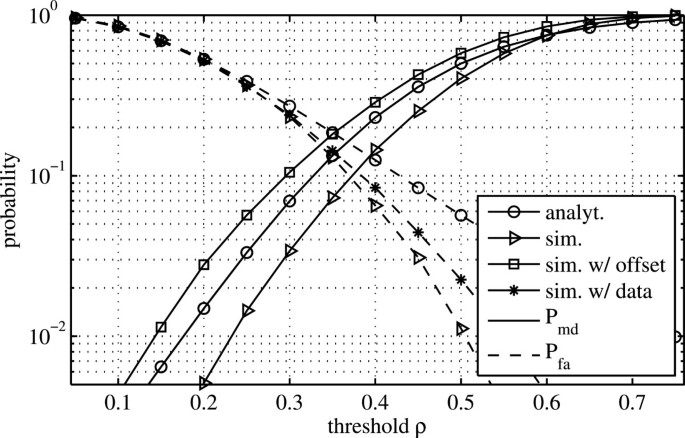
Theoretically derived P md and P fa and simulation results for W=32 and in an AWGN channel.
Figure 5 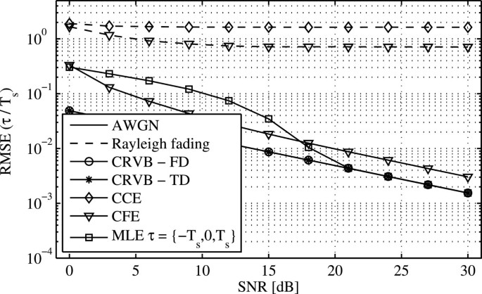
Comparison of the theoretically derived RMSE of the STO τ with simulation results. The STO is normalized with respect to the sample time T s . The CCE for AWGN shows no error for the given SNR range. Furthermore, the performance floor of the CFE as a result of the self-interference has no effect on the estimation for the given SNR range.
Figure 6 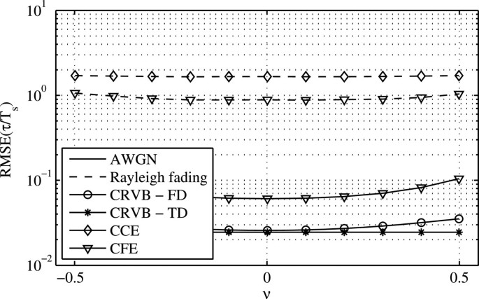
Analysis of influence of ν on STO estimation performance of CFE and CCE at an SNR of 6 dB. The CCE in AWGN results in no observed error due to the integer trial values of .
Figure 7 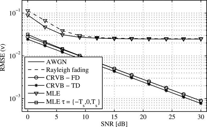
Comparison of the theoretically derived RMSE of the estimation of the CFO ν with simulation. The CFO is normalized with respect to the subchannel spacing.
Figure 8 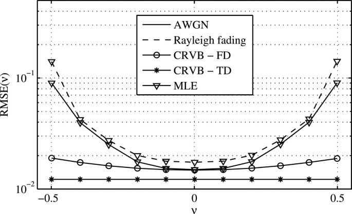
Analysis of influence of ν on CFO estimation performance of MLE at an SNR of 6 dB.
-
The prototype filter p[n T s ] is designed following the frequency sampling approach to filter design. We use the filter introduced in [16], which is defined by the overlapping factor β=3 and the corresponding design parameter equal to 0.91697069.
-
The STO τ and the normalized CFO ν are assumed to be uniformly distributed in the range of {−T/4+T s ,T/4−T s } and (−0.5,0.5), respectively, if not otherwise stated. For the case of Rayleigh fading, τ refers to the delay of the rounded mean path delay of each realization of the channel.
-
The Rayleigh fading channel is emulated with an exponential-decaying power delay profile according to with n∈{0,⋯,K/4−1}. A normalization of the power delay profile with is applied. The channel is static for each run but is varied between runs.


4.1 Frame detection
Beginning with the previously derived analytical expressions for Pmd and Pfa, Figure 4 shows the comparison of the analytical with the simulation-based results. The analytical derivation of Pmd over the threshold value ρ is based on the assumption that the STO and CFO are small. To take the influence of the offsets into account, two scenarios are considered in the simulations. Firstly, the Pmd for the ideal case with no offset is evaluated, shown as the lower solid curve in Figure 4. Secondly, the offset-afflicted Pmd is plotted, represented by the upper solid curve. The curve of the analytically derived performance is lying in between these two. The analytical and zero-offset results well agree with the results for the corresponding time domain metric presented in [13]. Furthermore, it shows that in the presence of STO and CFO, the detection rate degrades due to the amplitude degradation of the received preamble symbols and the introduction of interference.
The analytically derived Pfa, which assumes the presence of pure noise, is given by the upper dashed curve in Figure 4. As observed from this figure, it provides a pessimistic performance prediction compared to the outcome of the simulations, given by the two lower dashed curves. The difference stems from the approximations made during the derivation of Pfa. For the simulation results, two different scenarios are differentiated here. The lower dashed curve states the detection performance in the presence of pure noise, whereas the dashed line in the middle specifies the case that offset-afflicted payload symbols are received. For frame detection in time domain, these two cases are considered equal, because the time domain multicarrier signal is assumed to be distributed according to a normal distribution, yielding similar characteristics as the noise [13]. For the frequency domain approach, however, this assumption is no longer valid, as indicated by the simulation results.
4.2 Offset estimation
The evaluation of the estimation performance for STO and CFO, which follows the frame detection process, is discussed in this section. The analytical derivation of the CRVB of the time domain estimation method, presented in [2] and referred to as CRVBTD, is introduced here to compare the lower bounds of the two approaches. The CRVBTD can be written as [2]
and
A different preamble structure is used, which is defined as with the pilot symbols and . dk,m needs to be repeated with m={0,⋯,2(β+2)−1} to create two identical signal parts in the time domain. As can be seen from (37), the CRVBTD(τ) is related to the set of subchannel indices , which are bearing the training symbols. The CRVBTD(ν) remains independent of it and only depends on the value W, as given in (38). To compare the obtained CRVB for frequency domain processing (36) with the CRVBTD of the time domain solution, they have to be normalized with respect to the overall power used. Taking into consideration that OQAM-OFDM symbols are shifted half a symbol period T/2, the resulting SNR is
where Psample is the power per sample and Pnoise represents the noise power. For the boosted pilots of the frequency domain preamble, the ratio of Psymbol and Pnoise per utilized subchannel is
given that , as derived in Appendix 1. The resulting processing gain of the frequency domain-based approach can be intuitively explained: By processing only the subchannels bearing a pilot, half the noise power present at unoccupied subchannels is abandoned and not used in the metric, whereas in the time domain metric, no equivalent noise filtering takes place. The second parameter, which is important for the evaluation of the CRVB and comparison between the time and frequency domain methods, is the number of observations. While the time domain estimate is based on WTD=2K samples, we have only W=K u observations for the frequency domain method. The relation between these two yields
Hence, the sparse preamble exhibits a loss of at least a factor of 2 in number of observations W, affecting the corresponding CRVB. For K u =K, however, it can be shown that the gains and losses compensate each other. It follows from this consideration that the frequency domain CRVB is close to its time domain counterpart, as confirmed by looking at the two lower solid curves in Figure 5. In Figure 5 and as well in Figure 7, the CRVB is shown for τ=0 and ν=0.
The MLE for the STO (29) can achieve the CRVB for high SNR values for the limited estimation range of −T s ≤τ≤T s and in AWGN conditions. The results indicate that the given and an SNR value of 21 dB are sufficient for the MLE to be unbiased and asymptotically optimal [15]. For verification of the derived CRVB, the MLE is evaluated only in AWGN conditions. The CFE approaches the CRVB but is suboptimal since a gap between the RMSE of the estimation and the theoretical bound persists even for high SNR values in case of AWGN. The CFE does not account for the subchannel index k in (30), as the MLE does in (28), and hence, it does not deploy the complete received information. The performance of the CFE is significantly lowered by the Rayleigh fading, which results from the spread of received power over multiple channel taps and the corresponding interaction between different paths at the pilot positions in the frequency domain. Additionally, the estimation is subject to rounding errors as the CFE estimates the mean delay of the channel, which is compared to the rounded mean delay of the channel. The CCE achieves a similar performance as the CFE for the given reasons but is not subject to rounding errors for the Rayleigh fading case. In the case of AWGN and for the given number of realizations, the CCE, based on the integer nature of the estimation , produces no error. This complies with the observation that the RMSE values of the closed-form estimators are well below the rounding threshold of 0.5, where rounding the residual error to the next integer would yield zero as well. Since Figures 2 and 3 clearly suggest that the CFO has the most dominant effect on the estimation performance, the influence of the CFO on the RMSE is investigated in Figure 6, where the performance of the CCE and the CFE is shown over fixed values of the ν while τ is spanning the complete range. In both cases, AWGN and Rayleigh fading, the estimation of τ only weakly depends on the CFO.
The proximity of CRVB and CRVBTD can as well be observed in Figure 7 where the RMSE of the CFO estimation is given. The CFO estimation in the frequency domain shows a slightly higher bound which is assumed to result from the different approximations used during derivation. As a verification of the derived CRVB, the MLE of the CFO is simulated with zero frequency offset and a small timing offset of −T s ≤τ≤T s . Figure 7 clearly shows that the MLE yields the derived CRVB, suggesting that the CRVBTD is too optimistic. The results for the MLE with offsets spanning the complete range show a performance approaching the CRVB for low SNR, while for higher values of the SNR, the RMSE runs into a performance floor. In Rayleigh fading environments, the CFO estimator exhibits almost the same performance as in the AWGN case and is only slightly degraded by the effects of the channel. The performance floor is mainly due to the remaining intrinsic interference from intercarrier interference between pilot symbols in the presence of frequency offsets and is the dominant impairment for high SNR, as Figure 8 indicates. The position of the performance floor is calculated in the Appendix 5 to be at 1.82×10⁻². Even though the CRVB degrades only slightly with increasing CFO, the difference between the CRVB and the MLE is 1 order of magnitude higher for the maximum CFO close to 0.5 compared to the case of zero CFO as a result of the intrinsic interference. For the case that the CFO is below 0.1, the MLE achieves the CRVB. This leads to the conclusion, that given |ν|<0.1, the resulting interference is sufficiently small to obtain an estimate close to the optimum.
4.3 Synchronization concepts
The results from Figure 8 suggest to consider two different concepts as outlined in Figure 9 and in the following list.
-
Concept 1. The demodulation of the received samples is only performed once, and CFO estimation and STO estimation are performed on the same, unsynchronized demodulated signal.
Figure 9 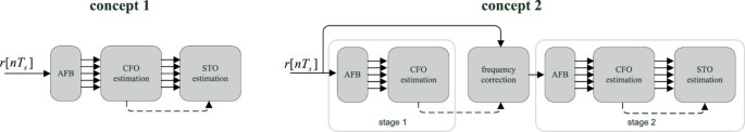
Different methods for frame detection and estimation using the core algorithms discussed. The analysis filter bank (AFB) describes the demodulation stage which provides the transition from time to frequency domain. Dashed lines indicate the passing of estimated CFO values, and solid lines indicate the flow of received samples in time domain (single path) or symbols in frequency domain (parallel paths).
-
Concept 2. After demodulation, the CFO is estimated, which will bring the residual CFO down to ±10% of the subchannel spacing as indicated in Figure 8. After correcting the CFO in the time domain based on the first estimate, the CFO can be estimated a second time, now yielding an error below 2% according to Figure 8, which will significantly lower the performance floor.The two concepts are assessed in terms of achievable RMSE in Figures 10 and 11 and by means of BER in Figure 12 for the two relevant STO estimators CFE and CCE. The frame structure used in the evaluation is the one described in Figure 1.
Figure 10 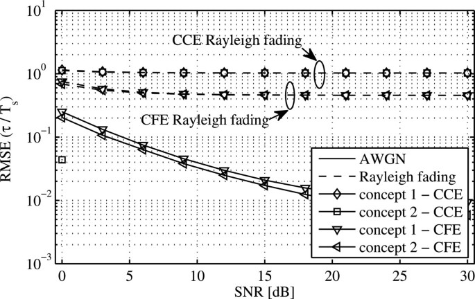
Performance evaluation of different STO estimation methods versus SNR.
Figure 11 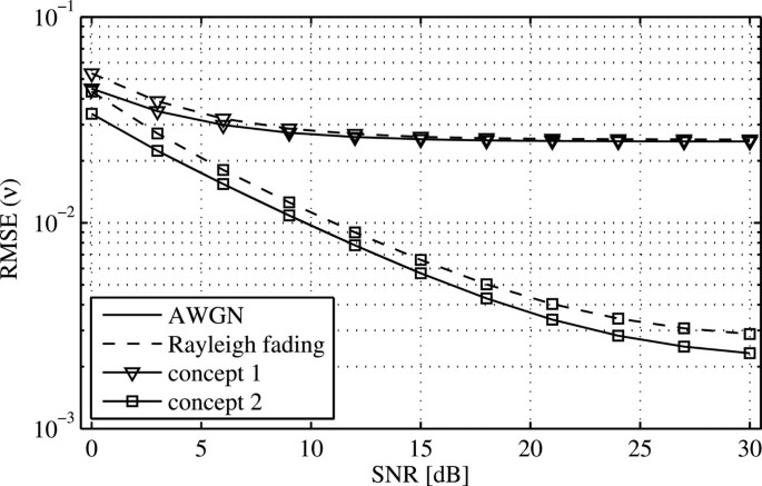
Performance evaluation of the CFO estimation for concepts 1 and 2 versus SNR.
Figure 12 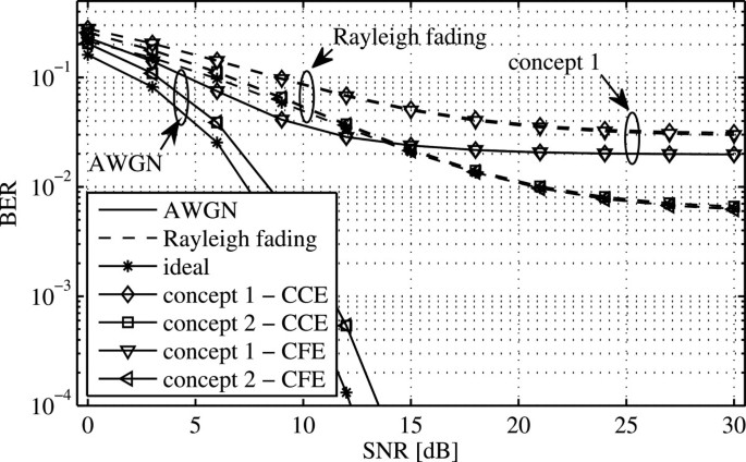
BER performance of the two concepts under AWGN and Rayleigh fading conditions. Each payload QAM symbol is modulated using a 4-QAM modulation alphabet.


In contrast to the previous evaluation of the core algorithms, outliers showing an absolute error greater than T/4 and 0.5 for the estimation of STO and CFO, respectively, are considered as falsely detected and are not included in the following results. The number of discarded estimations of this kind is well below 1% in the case of AWGN and below 5% in the case of Rayleigh fading channel conditions. The results from Figure 6 show only a weak influence of the CFO on the STO estimation. Given this observation, the difference between concepts 1 and 2 regarding the STO estimation does not vary significantly, which is as well indicated in Figure 10. In the case of concept 2 with CCE, one exception can be observed. Obviously, the additional consideration of the CFO to improve the estimation leads in some rare cases to timing errors due to an erroneous compensation of the CFO in (32) which could not be observed in the results for concept 1. In all cases, the additional payload leads to a worse estimation due to the increased interference. Figure 11 clearly shows that, in contrast to the STO estimation, concept 2 offers a significantly lower interference-induced performance floor for the CFO estimation. Comparing the results for concept 1 and concept 2, it can be concluded that concept 2 benefits from the smaller CFO after the second demodulation, confirming the results in the previous section. The evaluation of the BER, plotted in Figure 12, assumes perfect channel knowledge in combination with a one-tap zero-forcing equalizer to recover the data symbols, which are modulated using a 4-QAM symbol constellation. It is assumed that the channel is obtained at the preamble position, and the common phase error is zero at this position. The residual CFO after synchronization leads to a linearly increasing phase per OQAM-OFDM symbol, which affects the demodulation of the payload symbols. In general, it can be observed that the difference between the CFE and the CCE is not significant when it comes to BER. This can be explained by the ability of the channel equalizer to effectively reduce the distortion of the phase per subchannel caused by small timing offsets. On the contrary, residual frequency offsets result in a phase drift over time with a high impact on the constellation diagram at receiver side if they are not tracked. As a result, concept 1 approaches the BER floor at 2×10⁻² in both AWGN and Rayleigh fading conditions. The results for concept 2 indicate that the gain in CFO estimation accuracy is sufficient to get close to the ideal BER performance for AWGN and to match it in Rayleigh fading environments.
As a result, it can be shown that frequency domain synchronization methods can cope with the offset-afflicted self-interference and offer a system performance that reaches the ideal case. To achieve this, it is sufficient to estimate and compensate for the CFO in an initial stage to further improve the CFO estimation, while the STO only needs to be estimated in the second stage.
4.4 Computational complexity
The necessary demodulation process for frequency domain processing imposes additional complexity to the system compared with common time domain methods. In this section, the cost of frequency domain processing and the related algorithms is evaluated in terms of the number of complex multiplications needed to obtain frame detection and synchronization. Operations that involve additions are assumed to take significantly less resources than multiplications and are thus not considered in the complexity analysis. This holds similarly for taking the absolute value and the angle of a complex number. Furthermore, divisions and real multiplications are treated as complex multiplications. The number of complex multiplications C is calculated for K/2 processed samples in the time domain which corresponds to one OQAM-OFDM symbol in the frequency domain. For the calculation of the complexity, K2=K/2 is assumed. The complexity for the demodulation step in combination with the frame detection is labeled CAFB. As a time domain reference scheme, a Schmidl & Cox-like metric [12] is chosen that can be used for frame detection and STO and CFO estimation. Its complexity is labeled CS&C. The complexity for the different STO estimation schemes CCFE i and CCCE i using either concept 1 or 2 is indicated accordingly.
The complexity is calculated with regard to K/2 processed samples. In the case of Schmidl & Cox, three complex multiplications are considered per processed sample for frame detection and STO and CFO estimation. Furthermore, from the frame detection metric used in the frequency domain processing, the CFO estimation can be directly calculated and the CFO estimation is considered to add no complexity here. The STO and CFO estimation is not performed on each block of K/2 samples but is triggered by the frame detection and is therefore processed per detected frame.
From Figure 13, it becomes apparent that, compared to the time domain metric, the frequency domain processing adds complexity just in demodulation and frame detection by a factor of 5. Using concept 2 adds a significant amount of additional resources needed for both STO estimators, CFE and CCE, by involving a frequency correction of the (2β+2)K/2 samples in the time domain and their successive demodulation. The number of multiplications needed for the CFE increases moderately with K for both concepts, whereas the complexity increases significantly for the CCE. This makes the closed-form STO estimator a good choice, in particular when considering the fact that there is no significant performance difference in BER for the two STO estimators.

Computational complexity. Computational complexity of frame detection and STO and CFO estimation in number of complex multiplications per processed OQAM-OFDM symbol.
5 Conclusions
In this contribution, we showed that frame detection and synchronization can efficiently and satisfactorily be achieved in the frequency domain, taking advantage of the analysis filter bank at the receiver side. Our analysis concludes that, in theory, frequency domain synchronization schemes achieve a similar performance as time domain approaches. This is indicated by the Cramér-Rao bounds that have been derived as part of this work. In practice, the results reveal that the performance of the algorithms strongly depends on the interference introduced by the carrier frequency offset. This drawback is removed effectively by the introduction of a frequency correction stage, leading to a bit error rate that is close to the ideal one. Even though the complexity analysis demonstrates that the frequency domain approach calls for a significantly higher computational effort, its advantage lies in shared spectrum scenarios where frequency bands, which are assigned to individual users or systems, can be synchronized and processed separately.
Appendix 1
Definition of C Ψ
The properties of the noise samples after passing through the analysis filter bank are derived here. The time domain noise vector n=[⋯,η[(i−1)T s ],η[i T s ],η[(i+1)T s ],⋯ ] with zero mean and circular symmetric Gaussian noise leads to the diagonal covariance matrix C n
Passing through the analysis filter bank, the noise samples are getting transformed. For the derivation, the filter bank is formulated in the extended DFT representation, as described in [17]. It utilizes a DFT matrix W of size β K with subsequent weighting and summation of the frequency bins by P to obtain the subchannel symbols. P is constructed by circularly shifting the vector , about β entries to the right for each row, starting with .
The filter coefficients are derived from the frequency sampling technique presented in [16]. Using this formulation, the covariance matrix of the filtered noise is
with the matrix R
R has only non-zero entries on the first off-diagonals, which are occupied by some value |α|<1. Under the assumption that p[n T s ] is, in good approximation, a perfect reconstruction pulse shape that overlaps only with the subchannels directly adjacent to itself, P PH=I+R holds.
To distinguish between time and frequency domain noise energy, is renamed to for in (50). Considering the structure of the preamble with only every second subchannel occupied, the noise that adds to the received pilot symbols after the analysis filter bank can still be considered white Gaussian noise. Furthermore, it is independent of the offset that affects the received pilot symbols. This can also be understood intuitively by looking at the transfer function of the prototype filter which expands only over adjacent subchannels. Therefore, the relevant covariance matrix is C Ψ , as defined in (25).
Appendix 2
Derivations for P md and P fa
For the derivation of the Pmd and Pfa, the distribution of the metrics need to be calculated. Using the signal model from (8), the correlation metric C b [m], derived from in (13), can be written as
Setting m=0 and discarding the index m for simplicity in C b [m], the metric C b can be written in matrix notation as
which can be approximated for small values of τ and ν, resulting in a i ≈1 and E=I. With the help of (4), it leads to
ϕ is set to zero without loss of generality. For further analysis, C b is split into its real part and its imaginary part , and their statistical properties are evaluated independently for each summand κ i , as described in [13]. It follows for κ1 that ℜ{κ1}=γ2 and I{κ1}=0. Given Ψ is white Gaussian noise and , κ2 and κ3 are i.i.d. normal distributed with the variances and mean values according to
Using the central limit theorem for the evaluation of κ4 yields
Merging these results ends up in a normal distributed PDF of and according to
Taking the absolute value of C b according to results in to be Rician-distributed. For large values of W, the approximation can be made due to the dominant influence of on the distribution.
From (14), by discarding the index m and using the matrix notation, it follows that
Thereby, ϑ1=γ2 and . ϑ3 can be reformulated as
and modeled as a chi-square distribution according to . The scaled chi-square distribution can be transformed into a gamma distribution, which itself can be approximated by a normal distribution with for a large number of W. By using the same steps, it follows for ϑ4 that . Merging the results under the verified assumption that the covariances of ϑ i are zero leads to
The conditional PDF can be calculated with the help of [15], and its mean μ and variance σ2 are given by
with the covariance
After some calculations and with
the covariance is given by . Now (62) and (63) can be expressed as
and can be calculated depending on W and the ratio . The ratio corresponds to a signal-to-noise ratio per subchannel in the frequency domain.
Concerning the derivation of Pfa, adapting (57) and (58) to match (18) directly results in the following distributions for the real and imaginary parts:
Modifying the decision rule to utilize the squared absolute value of C Ψ results to be chi-square distributed with 2 degrees of freedoms according to . Then, the relation between the chi-square and the gamma distribution leads to
From (61), it follows analogously for Q Ψ that
and f(Q Ψ ) can be used to calculate the Pfa from (21). It has been shown in [13] that is only a scaling factor for and f(Q Ψ ) resulting in Pfa to be independent of the noise power.
Appendix 3
Regularity condition
Before beginning the calculation of the Cramér-Rao vector bound, the fulfillment of the regularity condition
needs to be assured. Thereby, (24) leads to
with Ψ=[Ψ1,Ψ2,⋯,Ψ W ]T as defined in (8). It follows that
In the last calculation step, the expectation can be taken for each coefficient of the product ∂ Ψ w /∂ v i Ψ w independently because ∂ Ψ w /∂ v i and Ψ w are statistically independent. With , the regularity condition is fulfilled and the CRVB can be calculated for the given problem.
Appendix 4
Fisher information matrix
The Fisher information matrix F is calculated from (34) and application of the log likelihood function (24). The matrix entry related to the estimation of τ, F(1,1), leads to the expression
which is simplified by replacing with Ψ and evaluation of the derivation. Further assessment of the expression leads to
When taking the expectation, only the last summand results in a non-zero contribution because E[(Ψk,m)2]=0 and . It follows that
Replacing with and EHE=I produces
The upper and the lower half of the matrices can be treated separately because the corresponding symbols b0 and b2 are considered mutually independent. When discarding the matrix notation and making use of , (77) results in
with W the number of observations per symbol equal to the elements used in the set of subchannels .
Replacing with in (76) and further calculation yield
For the derivation of F(3,3), the replacement of with in (74) leads to
Using the same argumentation regarding Ψ as for the calculation of (76), it follows that
The off-diagonals are given in (82), (83), and (84). F(1,2)=F(2,1) is derived from
F(1,3)=F(3,1) and F(2,3)=F(3,2) are derived in analogy and result in
Appendix 5
Performance floor calculation
Given the preamble structure from (4), the minimum achievable estimation error only depends on the pulse shape p[n T s ]. Therefore, the RMSEmin(ν) can be determined by looking at the ambiguity functions for a single subchannel averaged over the offset range and possible combinations of the preamble sequence bk,m from (4) according to
with the CFO estimation error ε ν (τ,ν,c) and the number of possible combinations of the BPSK preamble sequence nc. For the calculation of the minimum achievable RMSE, the influence from four surrounding subchannels is taken into account to capture the interference in the case of frequency offsets. The error ε ν (τ,ν,c) depends on the combination index c and the offsets τ and ν and is defined as the difference in phase between the interference-free estimate and the interference-afflicted estimate (a2(τ,ν)+ι2(τ,ν,c))∗(a0(τ,ν)+ι0(τ,ν,c))
The interference from the neighboring preamble symbols, summarized in the terms ι i (τ,ν,c), is calculated as
In the considered case of K=32 and the pulse shape p[n T s ], RMSEmin(ν) yields 1.82×10⁻², which is close to the RMSE value that the performance floor in Figure 7 approaches.
References
Farhang-Boroujeny B: OFDM versus filter bank multicarrier. IEEE Signal Process. Mag 2011, 28(3):92-112.
Fusco T, Petrella A, Tanda M: Data-aided symbol timing and CFO synchronization for filter bank multicarrier systems. IEEE Trans. Wireless Comm 2009, 8(5):2705-2715.
Hidalgo Stitz T, Ihalainen T, Renfors M: Practical issues in frequency domain synchronization for filter bank based multicarrier transmission. In Proceedings of the 3rd International Symposium on Communications, Control and Signal Processing (ISCCSP 2008). IEEE, St Julians, Malta, 12–14 March 2008; 411-416.
Stitz TH, Ihalainen T, Viholainen A, Renfors M: Pilot-based synchronization and equalization in filter bank multicarrier communications. EURASIP J. Adv. Signal Process 2010, 2010: 1-18.
Saeedi-Sourck H, Sadri S: Frequency-domain carrier frequency and symbol timing offsets estimation for offset QAM filter bank multicarrier systems in uplink of multiple access networks. Wireless Pers. Comm 2012, 70(2):601-615.
Amini P, Farhang-Boroujeny B: Packet format design and decision directed tracking methods for filter bank multicarrier systems. EURASIP J. Adv. Signal Process 2010, 2010: 1-14.
Saeedi-Sourck H, Sadri S, Wu Y, Farhang-Boroujeny B: Near maximum likelihood synchronization for filter bank multicarrier systems. IEEE Wireless Commun. Lett 2013, 2(2):235-238.
Thein C, Fuhrwerk M, Peissig J: Frequency-domain processing for synchronization and channel estimation in OQAM-OFDM systems. In Proceedings of the 14th Workshop on Signal Processing Advances in Wireless Communications (SPAWC 2013). IEEE, Darmstadt, Germany, 16–19 June 2013; 634-638.
Siohan P, Siclet C, Lacaille N: Analysis and design of OFDM/OQAM systems based on filterbank theory. IEEE Trans. Signal Process 2002, 50(5):1170-1183. 10.1109/78.995073
Javaudin J-P, Lacroix D, Rouxel A: Pilot-aided channel estimation for OFDM/OQAM. In Proceedings of the 57th IEEE Semiannual Vehicular Technology Conference (VTC 2003-Spring), vol. 3. IEEE, Jeju, Korea, 22–25 April 2003; 1581-15853.
Kofidis E, Katselis D, Rontogiannis A, Theodoridis S: Preamble-based channel estimation in OFDM/OQAM systems: a review. Signal Process 2013, 93(7):2038-2054. 10.1016/j.sigpro.2013.01.013
Schmidl TM, Cox DC: Robust frequency and timing synchronization for OFDM. IEEE Trans. Comm 1997, 45(12):1613-1621. 10.1109/26.650240
Schellmann JM: Multi-user MIMO-OFDM in practice: enabling spectrally efficient transmission over time-varying channels. PhD thesis, Technische Universität Berlin. 2009.
Moose PH: A technique for orthogonal frequency division multiplexing frequency offset correction. IEEE Trans. Comm 1994, 42(10):2908-2914. 10.1109/26.328961
Kay SM: Fundamentals of Statistical Signal Processing: Estimation Theory, vol. 1. Prentice-Hall PTR, New Jersey; 1993.
Viholainen A, Ihalainen T, Stitz TH, Renfors M, Bellanger M: Prototype filter design for filter bank based multicarrier transmission. In Proceedings of the 17th European Signal Processing Conference (Eusipco 2009). EURASIP, Glasgow, Scotland, 24–28 August 2009; 1354-1358.
Bellanger M: FBMC physical layer: a primer. PHYDYAS; 2010. . http://www.ict-phydyas.org/teamspace/internal-folder/FBMC-Primer_06-2010.pdf
Author information
Authors and Affiliations
Corresponding author
Additional information
Competing interests
The authors declare that they have no competing interests.
Authors’ original submitted files for images
Below are the links to the authors’ original submitted files for images.
Rights and permissions
Open Access This article is distributed under the terms of the Creative Commons Attribution 2.0 International License (https://creativecommons.org/licenses/by/2.0), which permits unrestricted use, distribution, and reproduction in any medium, provided the original work is properly cited.
About this article

Cite this article
Thein, C., Schellmann, M. & Peissig, J. Analysis of frequency domain frame detection and synchronization in OQAM-OFDM systems. EURASIP J. Adv. Signal Process. 2014, 83 (2014). https://doi.org/10.1186/1687-6180-2014-83
Received:
Accepted:
Published:
DOI: https://doi.org/10.1186/1687-6180-2014-83