Distributed weighted sum-rate maximization with multi-cell uplink-downlink throughput duality

Abstract

The weighted sum-rate maximization (WSRMax) problem is important for the radio resource allocation in wireless networks. In this paper, we focus on solving the WSRMax optimization problem in a Home eNodeB (HeNB) wireless network for the multiple input single output (MISO) downlink transmission. Based on an ameliorated max-min multi-cell uplink-downlink throughput duality, we design a distributed algorithm which contains Loop1 and Loop2 associating with the max-min procedure, respectively. Especially, in Loop2 procedure, we propose a new distributed iteration scheme with the complete proof. During the implementation of the proposed algorithm, randomly deployed HeNBs only need to share information with their neighboring nodes. Simulation results show that the two processes can converge to a stable state, and the network capacity is dramatically improved with the coordination among HeNBs.

1 Introduction

Since macro networks show poor indoor coverage capability, Home eNodeB (HeNB) network has been advocated to remedy this defect. Benefiting from the close proximity of transmitters and receivers, the HeNB network can provide high link quality for users. On the other hand, the deployment of HeNBs is flexible in accordance with consumers’ requirements. However, it is difficult to manage such a flexible network in a centralized manner. Thus, radio resource allocation with distributed coordinations among HeNBs is expected. Furthermore, as a promising technology, multi-antenna can improve the network throughput dramatically, while resulting in a more complex interference management problem [1-3]. Therefore, it is a challenging task to optimize the resource allocation in HeNB networks equipped with multiple antennas. It is worth noting that the radio resource allocation problem is generally formulated as a weighted sum-rate maximization (WSRMax) problem, which has attracted a lot of attentions recently.

Literature review. Several approaches to optimize the WSRMax problem in multi-antenna systems have been proposed. Some of them are centralized methods which include the monotonic optimization method [4,5], uplink-downlink signal-to-interference-plus-noise-ratio (SINR) duality [6-8], and branch-and-bound technique [9]. Nowadays, a great interest has been sparked in developing distributed methods. In [10-12], the problem is solved in distributed ways based on the pricing mechanism. However, the method in [10] splits the channel allocation process with beamforming and power optimization, and both methods in [11,12] are restricted to single user per cell scenario. In [13], the method iterative coordinated beamforming (ICBF) makes use of the necessary optimality condition for the WSRMax to design distributed solutions without completed theoretical proofs, and its results elucidate that the coordination can provide considerable gains. With the block coordinate descent (BCD) method proposed in [14,15], a single base station is optimized while others are fixed at each iteration. In [16], a distributed algorithm relying on weighted minimum mean square error (WMMSE) problem is proposed. In order to execute the WMMSE algorithm, each terminal needs to estimate the signal covariance and feed back certain prices to the base station. Authors in [17] incorporate primal decomposition subgradient method with the second-order cone programming (SOCP) and propose a distributed approach. In this algorithm, each base station has to complete the complexity SOCP programming in certain procedure. These previous works show that the coordinated beamforming is beneficial for system performance. Recently, the multi-cell uplink-downlink throughput duality theory is proposed as a novel tool to solve the WSRMax problem in [18] for the first time. With such duality, the downlink beamforming can be optimized with low complexity according to the virtual uplink structure [19,20]. However, as far as we know, a distributed approach for solving the WSRMax problem with the duality is still vacant.

In this paper, by utilizing the novel duality theory, we optimize the multi-antenna HeNB network’s capacity with a coordinated beamforming strategy. To avoid too much information exchange during coordinations, HeNBs are constrained to only share information with their neighbors. The detailed contributions of this paper are stated as follows.

• We ameliorate multi-cell uplink-downlink throughput duality into the multi-cell multi-user multi-channel network with an undirected graph.

• The non-deterministic polynomial time (NP)-hard property of WSRMax problem [1] impedes the use of convex methods as well as the virtual uplink structure. Therefore, we use the successive convex approximation technique and the ameliorated virtual uplink structure to circumvent the non-convexity. With the max-min dual structure, we design a distributed algorithm with two loops. In Loop1, the distributed algorithm based on Lagrangian primal-dual subgradient (DLPDS) algorithm [21] is utilized to maximize the virtual uplink power problem. In Loop2, we propose a new distributed iteration scheme to solve the virtual uplink noise programming which posses a separable structure. With the above two process, we not only optimize the beamforming vector with low complexity Rayleigh-Ritz quotient criterion but also find a feasible virtual uplink SINR. With the virtual uplink SINR, the real feasible downlink SINR can be accessed for the strong duality between them.

The remainder of this paper is organized as follows. Section 2 is devoted to the system model and problem formulation. In Section 3, the distributed algorithm is proposed and analyzed in detail. Numerical results confirm the convergence of the proposed algorithm in Section 4. Section 5 concludes this article.

2 System model and problem formulation

In Figure 1, a HeNB network is depicted as an undirected graph $\mathcal {G}\left (\upsilon,\varepsilon \right)$, where the set of HeNBs is denoted as υ={1,2,…,N} and ε⊂υ×υ is the set of edges. With a given interference threshold, each HeNB maintains neighboring relationships with other nodes, i.e, if the interference between two HeNBs exceeds the threshold, their neighbor relationships will be established. In this bipartite network, an edge e _il =e _li ∈ε denotes HeNB i and HeNB l are neighbors, where i,l∈υ. Neighboring HeNBs can exchange information with each other on this edge. For simplicity, the neighbor set of HeNB i (including itself) is defined as subset ${{\mathcal {N}}_{i}}$, and the corresponding cardinality is ${{N}_{i}}=\left | {{\mathcal {N}}_{i}} \right |$. Each HeNB is assumed to be equipped with N _t transmit antennas, while each home user equipment (HUE) has a single receiving antenna. Both HeNBs and HUEs are randomly deployed, and the whole network works in time division duplex (TDD) mode. For HeNB i, there are K _i connected HUEs. Thus, the total number of HUEs can be expressed as $K={\sum \nolimits }_{i=1}^{N}{{{K}_{i}}}$. Each HeNB manages Q downlink channels, and the channel state information (CSI) is assumed to be perfectly known by HUEs. All HUEs can reuse the same frequency resource, and the received signal y _i,j (q) at the jth HUE served by the ith HeNB on qth channel is given by:

$$ \begin{aligned} {y_{i,j}}\left(q \right) =&\; \sqrt {{p_{i,j}}\left(q \right)} {\mathbf{h}}_{i,i,j}^{H}\left(q \right){{\mathbf{w}}_{i,j}}\left(q \right){s_{i,j}}\left(q \right) + {z_{i,j}}\left(q \right)\\ &+ {\sum\nolimits}_{l \ne j}^{{K_{i}}} {\sqrt {{p_{i,l}}\left(q \right)} {\mathbf{h}}_{i,i,j}^{H}\left(q \right){{\mathbf{w}}_{i,l}}\left(q \right){s_{i,l}}\left(q \right)}\\ &+\sum\limits_{m \ne i}^{{N_{i}}} {\sum\limits_{n}^{{K_{m}}} {\sqrt {{p_{m,n}}\left(q \right)}} } {\mathbf{h}}_{m,i,j}^{H}\left(q \right){{\mathbf{w}}_{m,n}}\left(q \right){s_{m,n}}\left(q \right), \end{aligned} $$

((1))

Figure 1

System model of randomly deployed HeNB networks.

where q is the channel index, p _i,j (q) is the transmit power sent from the ith HeNB to the jth HUE on the qth channel, ${{\mathbf {w}}_{i,j}}\left (q \right)\in {{\mathbb {C}}^{{{N}_{t}}\times 1}}$ represents the corresponding beamforming vector, ${{\mathbf {h}}_{m,i,j}}\left (q \right)\in {{\mathbb {C}}^{{{N}_{t}}\times 1}}$ is the associated channel between the mth HeNB and the jth HUE served by the ith HeNB, and z _i,j (q) is the additive white Gaussian noise with the variance $E\left \{ {{\left | {{z}_{i,j}} \right |}^{2}} \right \}={\sigma _{n}^{2}}$.

The downlink WSRMax problem with power constrains is generally defined as:

$$ \begin{aligned} &\mathop {\max }\limits_{{\mathbf{p}}, {\mathbf{w}}} {{\sum\nolimits}_{i}^{N}} {{{\sum\nolimits}_{q}^{Q}} {{\sum\nolimits}_{j}^{{K_{i}}} {\log \left[ {1 + \gamma_{i,j}^{\text{DL}}\left(q \right)} \right]}} } \\ &\hspace{8pt} s.t {{\sum\nolimits}_{q}^{Q}} {{\sum\nolimits}_{j}^{{K_{i}}} {{p_{i,j}}\left(q \right)} \le {P_{\max }}},\; \forall i = 1,\ldots,N;\\ & {\text{tr}}\left({\mathbf{w}}_{i,j}^{H}{\mathbf{w}}_{i,j}\right)=1,\; {p_{i,j}}\left(q \right) \ge 0,\\ &\forall i = 1,\ldots,N;\;\forall j = 1,\ldots,K;\;\forall q = 1,\ldots,Q, \end{aligned} $$

((2))

where the downlink SINR $\gamma _{i,j}^{\text {DL}}\left (q \right)$ is:

$${} {\fontsize{8.8pt}{9.6pt}\selectfont{\begin{aligned} \gamma_{i,j}^{\text{DL}}\left(q \right) = \frac{{{p_{i,j}}\left(q \right){{\left| {{\mathbf{h}}_{i,i,j}^{H}\left(q \right){{\mathbf{w}}_{i,j}}\left(q \right)} \right|}^{2}}}}{{{\sigma_{n}^{2}} + {\sum\nolimits}_{m = 1}^{{N_{i}}} {{\sum\nolimits}_{\left({m,n} \right) \ne \left({i,j} \right)}^{{K_{m}}} {{p_{m,n}}\left(q \right){{\left| {{\mathbf{h}}_{m,i,j}^{H}\left(q \right){{\mathbf{w}}_{m,n}}\left(q \right)} \right|}^{2}}}}}}, \end{aligned}}} $$

and P _max is the upper bound of the total transmit power. Problem (2) is proved to be an NP-hard problem, so it is very difficult to solve the beamforming vector directly.

3 Distributed algorithm derivation

Due to the NP-hard feature of the WSRMax problem shown in (2), the global optimal cannot be guaranteed [1]. We sequentially try to solve problem (2) with a lower bound approximation. Nevertheless, the lower bound approximation is still non-convex for the coupled beamforming vectors in the individual HeNB objective function. Furthermore, we transform the approximation into a virtual uplink structure with the uplink-downlink throughput duality. Because virtual uplink problem can be transformed into log-sum-exp (LSE) convex problem, it can be solved more efficiently. Moreover, the downlink beamforming vector can be updated with a low complexity Rayleigh-Ritz quotient criterion. Based on the max-min virtual uplink problem, we first apply DLPDS into Loop1 and propose a new distributed iteration scheme in Loop2 with the complete proof. After that, each HeNB not only obtains the downlink beamforming vectors for its HUEs but also calculates the feasible optimal downlink SINR as a result of the strong duality. With the feasible downlink SINR, each HeNB can assign the downlink transmit power easily. For the clarity of the exposition, the proposed algorithm is denoted as distributed joint power, channel, and beamforming optimization (DJPCBO), and the structure is shown in Figure 2.

Figure 2

Block diagram of the proposed algorithm.

3.1 SCALE approximation of virtual dual uplink problem

As shown in [22], a lower bound approximation of log(1+z) is presented as follows:

$${} \log (1 + z) \ge \alpha \log (z) + \beta\;,\;\left\{ \begin{aligned} &\alpha = \frac{{{z_{0}}}}{{1 + {z_{0}}}},\\ &\beta = \log (1 + {z_{0}}) - \alpha \log ({z_{0}}). \end{aligned} \right. $$

((3))

Note that the inequality is tight at z ₀=z. When the optimal value z ^∗ of the lower bound is found, parameters α, β can be updated according to z ₀=z ^∗. Based on (3), the network sum-rate can be relaxed as:

$$ \begin{aligned} &\mathop {\max }\limits_{{\mathbf{p}}, {\mathbf{w}}} {{\sum\nolimits}_{i}^{N}} {{{\sum\nolimits}_{q}^{Q}} {{\sum\nolimits}_{j}^{{K_{i}}} {\left\{ {\alpha_{i,j}}\left(q \right){\log_{2}}\left[ {\gamma_{i,j}^{\text{DL}}\left(q \right)} \right] + {\beta_{i,j}}\left(q \right) \right\}}} } \\ &\hspace{8pt}s.t{C_{1}}:\;{{\sum\nolimits}_{q}^{Q}} {{\sum\nolimits}_{j}^{{K_{i}}} {{p_{i,j}}\left(q \right) \le {P_{\max }}} }, \;\forall i,i = 1,\ldots N;\\ &{C_{2}}:\;{p_{i,j}}\left(q \right) \ge 0\\ &\forall i,i = 1,\ldots N;\;\forall q,q = 1,\ldots Q;\;\forall j,j = 1,\ldots K. \end{aligned} $$

((4))

Lemma 1.

The Lagrangian dual problem of multi-cell multi-user downlink beamforming problem can be defined as:

$${} {\fontsize{8.6pt}{9.6pt}\selectfont{\begin{aligned} &\mathop {\min }\limits_{{{{\bar{\boldsymbol{\lambda }}}_{\mathbf{2}}}}} \mathop {\max }\limits_{{{{\bar{\boldsymbol{\lambda}}}_{\mathbf{1}}}}, {\mathbf{w}}} {{\sum\nolimits}_{i}^{N}} {{{\sum\nolimits}_{q}^{Q}} {{\sum\nolimits}_{j}^{{K_{i}}} {\left\{ {{\alpha_{i,j}}\left(q \right){{\log }_{2}}\left[ {\gamma_{i,j}^{\text{UL}}\left(q \right)} \right] + {\beta_{i,j}}\left(q \right)} \right\}}} } \\ &\hspace{2pt}s.t {C_{1}}:{{{{\bar \lambda }}}_{{{1}},i,j}}\left(q \right) \ge 0 \forall i,i = 1,\ldots N;\;\forall q,q = 1,\ldots Q;\;\forall j,j = 1,\ldots K\\ & {C_{2}}:{{{{\bar \lambda }}}_{{{2}},i}} \ge 0 \forall i,i = 1,\ldots N\\ & {C_{3}}:{{\sum\nolimits}_{i}^{N}} {{{\sum\nolimits}_{q}^{Q}} {{\sum\nolimits}_{j}^{{K_{i}}} {{{{{\bar \lambda }}}_{{{1}},i,j}}}} } \left(q \right) \le {{\sum\nolimits}_{i}^{N}} {{P_{\max }}} \\ & {C_{4}}:{{\sum\nolimits}_{i}^{N}} {{{{{\bar \lambda }}}_{{{2}},i}}{P_{\max }}} \le {\sigma_{n}^{2}}{{\sum\nolimits}_{i}^{N}} {{P_{\max }}}, \end{aligned}}} $$

((5))

with the virtual uplink SINR $\gamma _{i,j}^{\text {UL}}\left (q \right)$

$${} {\fontsize{8.6pt}{9.6pt}\selectfont{\begin{aligned} \gamma_{i,j}^{\text{UL}}\left(q \right) = \frac{{{{{{\bar \lambda }}}_{{{1}},i,j}}\left(q \right){{\left| {{\mathbf{w}}_{i,j}^{H}\left(q \right){{\mathbf{h}}_{i,i,j}}\left(q \right)} \right|}^{2}}}}{{{\bar{{\lambda }}_{{{2}},i}} + {\sum\nolimits}_{m = 1}^{{N_{i}}} {{\sum\nolimits}_{\left({m,n} \right) \ne \left({i,j} \right)}^{{K_{m}}} {{{{{\bar \lambda }}}_{{{1}},m,n}}\left(q \right){{\left| {{\mathbf{w}}_{i,j}^{H}\left(q \right){{\mathbf{h}}_{i,m,n}}\left(q \right)} \right|}^{2}}}} }}, \end{aligned}}} $$

where ${{\boldsymbol {\bar {\lambda }}}_{1}}\in {{\mathbb {R}}^{K\times Q}}$ is a matrix of dual variables associated with the constraint C ₃, and ${{\boldsymbol {\bar {\lambda }}}_{2}}\in {{\mathbb {R}}^{N\times 1}}$ is a vector of dual variables associated with power constraint C ₄. Therefore, the dual problem can be interpreted as a virtual uplink problem where ${{\boldsymbol {\bar {\lambda }}}_{1}}$ is the virtual uplink transmit power, and ${{\boldsymbol {\bar {\lambda }}}_{2}}$ is the virtual uplink thermal noise. The strong duality is held between (4) and (5); consequently, the downlink and dual uplink problem can achieve the same optimal point.

The proof of Lemma 1 is presented in Appendix A. Since the HeNB network is assumed to work in TDD mode where the uplink and downlink channels are reciprocal, the downlink channel information can be estimated via uplink measurement. When the optimal variables $\left \{ {{{{\bar {\lambda }}}}^{^{\ast }}}_{{1},i,j}(q) \right \}, \left \{ \mathbf {w}_{i,j}^{^{\ast }}(q) \right \} \left \{ {{{{\bar {\lambda }}}}^{^{\ast }}}_{{2},i} \right \}$ of (5) are obtained, it is easy to calculate the optimal uplink SINR $\gamma _{i,j}^{\text {UL}^{\ast }}(q)$. Due to the strong duality, the optimal downlink SINR $\gamma _{i,j}^{\text {DL}^{\ast }}(q)$ can be achieved via:

$$ {z_{0}} = \gamma_{i,j}^{\text{DL}^{\ast}}(q) = \gamma_{i,j}^{\text{UL}^{\ast}}(q). $$

((6))

The equality $\gamma _{i,j}^{\text {DL}^{\ast }}(q) = \gamma _{i,j}^{\text {UL}^{\ast }}(q)$ is hidden in the proof of Lemma 1.

In the following subsections, we will implement Loop1 algorithm to the maximization process and design Loop2 algorithm to figure out the minimization procedure.

3.2 Loop1 design: uplink power and beamforming optimization

In Loop1, the maximization problem about the virtual uplink power ${{\bar {\lambda }}_{1}}$ and the beamforming vector w under the fixed virtual noise ${{\bar {\lambda }}_{{2}}}$ can be interpreted as:

$${} \begin{aligned} &\mathop {\max }\limits{\!~\!}_{{{{{\boldsymbol{\bar \lambda }}}{\!~\!}_{{1}}}}, {\mathbf{w}}} {{\sum\nolimits}{\!~\!}_{i}^{N}} {{{\sum\nolimits}{\!~\!}_{q}^{Q}} {{\sum\nolimits}{\!~\!}_{j}^{{K_{i}}} {\left\{ {{\alpha_{i,j}}\left(q \right){{\log }{\!~\!}_{2}}\left[ {\gamma_{i,j}^{\text{UL}}\left(q \right)\left| {{\!~\!}_{{{{{\boldsymbol{\bar \lambda }}}{\!~\!}_{2}}}}} \right.} \right] + {\beta_{i,j}}\left(q \right)} \right\}}} } \\ & s.t {C_{1}}:{{{{\bar \lambda }}}{\!~\!}_{{{1}},i,j}}\left(q \right) \ge 0 \forall i,i = 1,\ldots N;\forall j,j = 1,\ldots K\\ & {C_{3}}:{{\sum\nolimits}_{i}^{N}} {{{\sum\nolimits}_{q}^{Q}} {{\sum\nolimits}{\!~\!}_{j}^{{K_{i}}} {{{{{\bar \lambda }}}{\!~\!}_{{{1}},i,j}}}} } \left(q \right) \le {{\sum\nolimits}{\!~\!}_{i}^{N}} {{P_{\max }}}. \end{aligned} $$

((7))

For fixed $\left \{ {\mathbf {w}_{\textit {ij}}} \right \}_{(i=1,\ldots N, j=1,\ldots K_{i})}$, (7) is still a non-concave function. Nevertheless, it can be transformed into a LSE problem, which is known as geometric programming [23], by substituting ${{{\bar \lambda }}_{1,i,j}}\left (q \right) = {e^{{x_{i,j}}\left (q \right)}}$.

$${} \begin{aligned} &\mathop {\min }\limits_{{\mathbf{x}}} {{\sum\nolimits}_{i}^{N}} {{{\sum\nolimits}_{q}^{Q}} {{\sum\nolimits}_{j}^{{K_{i}}} {\left\{ { - {\alpha_{i,j}} \cdot {{\log }_{2}}\left({\gamma_{i,j}^{\text{UL}}\left(q \right)\left| {{\!~\!}_{{{{{\boldsymbol{\bar \lambda }}}_{2}}}, {\mathbf{w}} }} \right.} \right) - {\beta_{i,j}}} \right\}}} } \\ &\hspace{5pt}s.t {C_{3}}:{{\sum\nolimits}_{i}^{N}} {{{\sum\nolimits}_{q}^{Q}} {{\sum\nolimits}_{j}^{{K_{i}}} {{e^{{x_{i,j}}\left(q \right)}}}} } \le {{\sum\nolimits}_{i}^{N}} {{P_{\max }}}. \end{aligned} $$

((8))

The constraint C ₃ can be deemed as the global constraint which is copied across HeNBs according to DLPDS algorithm. Furthermore, it can be observed that $\mathbf {x}\in {{\mathbb {C}}^{K\times Q}}$ is a global variable coupling among different objective functions and the constraint C ₃ in (8). The Lagrangian function of (8) can be expressed as:

$$ L\left({ {\mathbf{x}},y} \right) = {{\sum\nolimits}_{i}^{N}} {{L_{i}}\left({{\mathbf{x}},y} \right)}, $$

((9))

with the individual Lagrangian function of HeNB i

$$\begin{aligned} &L_{i}\left({{\mathbf{x}},y} \right)\\ &={\sum\limits_{q}^{Q}} {\sum\limits_{j}^{{K_{i}}} {\left\{ - {\alpha_{i,j}}\left(q \right){\log_{2}}\left[ {\gamma_{i,j}^{\text{UL}}\left(q \right)\left| {{\!~\!}_{{{{{\boldsymbol{\bar \lambda }}}_{2}}}, {\mathbf{w}} }} \right.} \!\right]\! - {\beta_{i,j}}\left(q \right) \right\}} }\\ &\quad+y\left[{{\sum\limits_{i}^{N}} {{\sum\limits_{q}^{Q}} {\sum\limits_{j}^{{K_{i}}} {{e^{{x_{i,j}}\left(q \right)}}}} } - {P_{\max }}} \right], \end{aligned} $$

where y is the Lagrange multiplier associated with the global constraint C ₃ in (8). With the above discussion, the DLPDS can be applied into (9) as follows:

$${} \left\{ \begin{aligned} &{\mathbf{v}}_{\mathbf{x}}^{i}(k) = {\sum\nolimits}_{j = 1}^{{N_{i}}} {{{a}_{ij}}{{\mathbf{x}}^{j}}\left(k \right)},\\ &{{v}}_{y}^{i}(k) = {\sum\nolimits}_{j = 1}^{{N_{i}}} {{{a}_{ij}}{{{y}}^{j}}\left(k \right)},\\ &{{\mathbf{x}}^{i}}\left({k + 1} \right) = {P_{\mathbf{X}}}\left[ {{\mathbf{v}}_{\mathbf{x}}^{i}(k) - \phi \left(k \right){\nabla_{\mathbf{x}}}{L_{i}}\left({{\mathbf{v}}_{\mathbf{x}}^{i}\left(k \right),{{v}}_{y}^{i}\left(k \right)} \right)} \right],\\ &{y^{i}}\left({k + 1} \right) = {P_{\text{Y}}}\left[ {{{v}}_{y}^{i}\left(k \right) + \phi \left(k \right){\nabla_{y}}{L_{i}}\left({{\mathbf{v}}_{\mathbf{x}}^{i}\left(k \right),{{v}}_{y}^{i}\left(k \right)} \right)} \right], \end{aligned} \right. $$

((10))

where x ^j(k) denotes the matrix from the jth HeNB associating with the Lagrangian multiplier y ^j(k) at the kth iteration. ϕ(k) is the diminishing step size with the increasing iteration k. A fast linear non-negative weight a _ij (satisfying ${{\mathbf {1}}^{\mathbf {T}}}\mathbf {a}={{\mathbf {1}}^{\mathbf {T}}}, \mathbf {1}\mathbf {a}=\mathbf {1},\mathbf {1}\in {\mathbb {C}^{N \times 1}}$) is adopted to approach the average $\left ({1}/{N}\; \right){\sum \nolimits }_{j=1}^{N}{{{\mathbf {x}}^{j}}\left (k \right)}$ such that HeNBs only communicate with their neighbors. P _X and P _Y denote Euclidean projection onto set X={x|x _i,j (q)≤log(N P _max),i=1,…,N;j=1,…,K _i ;q=1,…,Q} and Y={y|y≥0}, respectively. ∇ _x L _i (·,y) can be expressed explicitly as:

• if m==i

  $${\fontsize{8.6pt}{9.6pt}\selectfont{\begin{aligned} \frac{{\partial {L_{i}}}}{{\partial {x_{m,j}}\left(q \right)}} \!&= \! \frac{- {\alpha_{i,j}}\left(q \right)}{{\ln 2}}\\ &\quad+ \sum\limits_{t \ne j}^{{K_{i}}} { {\frac{{{\alpha_{i,t}}\left(q \right){e^{{x_{i,j}}\left(q \right)}}{{\left| {{\mathbf{w}}_{i,t}^{H}\left(q \right){{\mathbf{h}}_{i,i,j}}\left(q \right)} \right|}^{2}}{{\log }_{2}}e}}{{{{{\bar \lambda }}_{{2},i}}\! +\! \sum\limits_{m = 1}^{{N_{i}}} {\sum\limits_{\left({m,n} \right) \ne \left({i,t} \right)}^{{K_{m}}} \!\!\!\!\!{{e^{{x_{m,n}}\left(q \right)}}{{\left| {{\mathbf{w}}_{i,t}^{H}\left(q \right){{\mathbf{h}}_{i,m,n}}\left(q \right)} \right|}^{2}}}} }}}}\\&\quad+ y{e^{{x_{i,j}}\left(q \right)}}, \end{aligned}}} $$

• if m ≠ i,m ∈ N _i

  $${\fontsize{8.6pt}{9.6pt}\selectfont{\begin{aligned} \frac{{\partial {L_{i}}}}{{\partial {x_{m,n}}\left(q \right)}}\! &=\!\! \sum\limits_{j}^{{K_{i}}} { {\frac{{{\alpha_{i,j}}\left(q \right){e^{{x_{m,n}}\left(q \right)}}{{\left| {{\mathbf{w}}_{i,j}^{H}\left(q \right){{\mathbf{h}}_{i,m,n}}\left(q \right)} \right|}^{2}}{{\log }_{2}}e}}{{{{{\bar \lambda }}_{{2},i}} + \sum\limits_{m = 1}^{{N_{i}}} {\sum\limits_{\left({m,n} \right) \ne \left({i,j} \right)}^{{K_{m}}} {{e^{{x_{m,n}}\left(q \right)}}{{\left| {{\mathbf{w}}_{i,j}^{H}\left(q \right){{\mathbf{h}}_{i,m,n}}\left(q \right)} \right|}^{2}}}} }}} }\\&\quad+ y{e^{{x_{i,j}}\left(q \right)}}, \end{aligned}}} $$

• if m∉N _i

  $$\frac{{\partial {L_{i}}}}{{\partial {x_{m,n}}\left(q \right)}}=0. $$

Specifically, the subgradient ∇ _y L _i (x,·) can be denoted as:

$$ {\nabla_{y}}{L_{i}} = {\sum\nolimits}_{\text{i}}^{N} {{{\sum\nolimits}_{q}^{Q}} {{\sum\nolimits}_{j}^{{K_{i}}} {{e^{{x_{i,j}}\left(q \right)}}}} } - {{\sum\nolimits}_{i}^{N}} {{P_{\max }}}. $$

((11))

DLPDS algorithm can converge to the global optimal state such that each HeNB i can obtain the optimal matrix x via the consensus process. After obtaining the optimal uplink power, the optimal beamforming vector can be achieved according to quasiconcave Rayleigh-Ritz quotient programming regardless of strong duality [18-20]:

$$ \begin{aligned} &{\mathbf{w}}_{i,j}^ * \left(q \right)\! \propto\!\\ &v_{\text{max}} \!\left[\!\left(\sum\limits_{m}^{{N_{i}}}\! \!\! {\sum\limits_{(m,n)\neq(i,j)}^{{K_{m}}} \!\!\!\!{{{{\bar \lambda}}^{*}}_{1,m,n}\left(q \right){{\mathbf{h}}_{i,m,n}}\left(q \right){\mathbf{h}}_{i,m,n}^{H}}} \left(q \right)\right.\right.\\ &\quad\qquad+ \left.\left.{{\bar \lambda}}_{2,i}{{\mathbf{I}}_{{N_{t}} \times {N_{t}}}}\vphantom{\left(\sum\limits_{m}^{{N_{i}}}\! \!\! {\sum\limits_{(m,n)\neq(i,j)}^{{K_{m}}} \!\!\!\!{{{{\bar \lambda}}^{*}}_{1,m,n}\left(q \right){{\mathbf{h}}_{i,m,n}}\left(q \right){\mathbf{h}}_{i,m,n}^{H}}} \left(q \right)\right.} \right)^{- 1}\!\!\!\!{{\mathbf{h}}_{i,i,j}}\left(q \right){{\mathbf{h}}_{i,i,j}^{H}}\left(q \right)\!\vphantom{\left(\sum\limits_{m}^{{N_{i}}}\! \!\! {\sum\limits_{(m,n)\neq(i,j)}^{{K_{m}}} \!\!\!\!{{{{\bar \lambda}}^{*}}_{1,m,n}\left(q \right){{\mathbf{h}}_{i,m,n}}\left(q \right){\mathbf{h}}_{i,m,n}^{H}}} \left(q \right)\right.}\right], \end{aligned} $$

((12))

where v _max(·) is the dominant eigenvector that corresponds to the maximum eigenvalue of the inner matrix. With the relevant channel information, beamforming vector can be updated with the low complexity linear operation according to (12). The convergence between x and w in Loop1 can be interpreted by the block coordinate descent theory (P271 [24]). As shown in (10), HeNB i only needs to share matrix x ⁱ and Lagrange multiplier y within its subset.

3.3 Loop2 design: uplink noise optimization

The aim of Loop2 algorithm is to optimize the virtual noise ${\bar \lambda }_{2}$ under fixed ${{\bar \lambda }_{1}^{*}}$ and w ^∗ which are outputted from Loop1 by solving the underlying minimization problem with the closed subset ${{\mathbf {\chi }}_{i}} = \left \{ {{{\bar \lambda }_{2,i}}\left | {0 \le {{\bar \lambda }_{2,i}} \le N{\sigma _{n}^{2}}} \right.} \right \}, \forall i=1,\ldots,N$.

$$ \begin{aligned} &\mathop {\min }\limits_{\left\{ {{{{\bar \lambda }}_{2,i}}} \in {{\mathbf{\chi }}_{i}} \right\}} {{\sum\nolimits}_{i}^{N}} {{f_{i}}\left({{{{{\bar \lambda }}}_{2,i}}} \right)} \\ &s.t {C_{4}}:{{\sum\nolimits}_{i}^{N}} {{{{{\bar \lambda }}}_{{{2}},i}}{P_{\max }}} \le {\sigma_{n}^{2}}{{\sum\nolimits}_{i}^{N}} {{P_{\max }}}, \end{aligned} $$

((13))

where ${{f_{i}}\left ({{{{{\bar \lambda }}}_{2,i}}} \right)}$ represents a local objective function of HeNB i and is given by:

$${} {\fontsize{9.2pt}{9.6pt}\selectfont{\begin{aligned} {f_{i}}\left({{{{\bar \lambda}}_{2,i}}} \right) = {{\sum\nolimits}_{q}^{Q}} {{\sum\nolimits}_{j}^{{K_{i}}} {\left\{ {{\alpha_{i,j}}\left(q \right){{\log }_{2}}\left({\gamma_{i,j}^{\text{UL}}\left(q \right)\left| {{\!~\!}_{{{\bar \lambda}_{1}^{*}}, {{\mathbf{w}}^{*}} }} \right.} \right) + {\beta_{i,j}}\left(q \right)} \right\}}}. \end{aligned}}} $$

The convexity of ${f_{i}}\left ({{{{\bar \lambda }}_{2,i}}} \right)$ can be proved by checking its positive Hessian matrix, and the pointwise sum of a convex function is still convex. The coupling constraint C ₄ and separable structure of (13) prompt us to apply distributed alternating direction method of multipliers (ADMM) algorithm [25] into its dual problem. The dual problem of (13) can be explicitly expressed as:

$$ \begin{aligned} &\mathop {\max }\limits_{y} \hspace{5pt}{\sum\nolimits}_{i = 1}^{N} {{g_{i}}(y)} \\ &\hspace{3pt} s.t y \ge 0, \end{aligned} $$

((14))

where ${g_{i}}(y) = \mathop {\min }\limits _{{{{\bar \lambda }}_{2,i}}\in {\mathbf {\chi }}_{i}} \left [\, {{f_{i}}\left ({{{{\bar \lambda }}_{2,i}}} \right) + y{c_{i}}\left ({{{\bar \lambda }_{2,i}}} \right)} \right ]$ is the dual problem of (13) with Lagrange multiplier y, and ${c_{i}}\left ({{{\bar \lambda }_{2,i}}} \right)={{{{\bar \lambda }}_{2,i}}{P_{\max }} - {\sigma _{n}^{2}}{P_{\max }}}$ is the individual constraint. The artificial parameter {z _i } is introduced into (14) as a copy of y. Then, the following equivalent form is derived.

$$ \begin{aligned} &\mathop {\max }\limits_{y} \;{\sum\nolimits}_{i = 1}^{N} {{g_{i}}\left({{z_{i}}} \right)} \\ &\hspace{5pt}s.t\;\;\;{\kern 1pt} {z_{i}} = {z_{l}},\;\;\left({i,l} \right) \in \varepsilon, \\ &\forall i,l= 1,\ldots,N. \end{aligned} $$

((15))

We aim to design a distributed algorithm to solve the separable convex programming given by (13). To facilitate the derivation of the proposed algorithm, the neighbors of HeNB i are partitioned into two sets, which are called predecessors and successors. The set of predecessors of HeNB i includes the neighbors whose indexes are smaller than i, i.e., P(i)={l|e _li ∈ε,l<i}, and the cardinality is |P(i)|=P _i . The set of successors of HeNB i consists of the neighbors with the indexes which are larger than i, i.e., S(i)={l|e _il ∈ε,i<l} with the cardinality |S(i)|=S _i . Then, we apply the distributed ADMM to the dual function shown in (15), and we obtain (16).

In the distributed ADMM algorithm, the dual variable λ _il with the constraint z _i =z _l on edge is defined. Each HeNB i only own the dual variable λ _mi for m<i and updates the dual variable. Nevertheless, the optimal $\{{{\bar \lambda }}_{2,i}\}_{\{i=1,\ldots,N\}}$ are the objectives that we concern about, and the next lemma reveals the connection between ${{\bar \lambda }}_{2,i}$ and z _i .

Lemma 2.

Let (16a) be satisfied, then $\bar \lambda _{2,i}^{k + 1}$ can be uniquely attained by solving the following convex problem:

$$ \begin{aligned} \bar \lambda_{2,i}^{k + 1} &= \mathop {\arg \min }\limits_{{{\bar \lambda }_{2,i}} \in {{\mathbf{\chi }}_{i}}} \left\{ {f_{i}}\left({{{\bar \lambda }_{2,i}}} \right) + \frac{1}{{2\rho \left({{P_{i}} + {S_{i}}} \right)}}\right.\\ &\quad\qquad\qquad\times \left.{{\left\{ {\max \left[ {0,{c_{i}}\left({{{\bar \lambda }_{2,i}}} \right) + A_{i} + B_{i}} \right]} \right\}}^{2}} \vphantom{{f_{i}}\left({{{\bar \lambda }_{2,i}}} \right) + \frac{1}{{2\rho \left({{P_{i}} + {S_{i}}} \right)}}}\right\}. \end{aligned} $$

((17))

Moreover, the $z_{i}^{k + 1}$ can be obtained from $\bar \lambda _{2,i}^{k + 1}$:

$$ {z_{i}^{k+1}} = \max \left\{ {0,\frac{1}{{\rho \left({{S_{i}} + {P_{i}}} \right)}}\left[ {{c_{i}}\left({{{\bar \lambda }_{2,i}^{k+1}}} \right) + A_{i} + B_{i}} \right]} \right\}, $$

((18))

where A _i and B _i are defined as follows:

$$\left\{ \begin{aligned} &A_{i} = \sum\limits_{l \in S\left(i \right)} {\left({\rho {z_{l}^{k}} - \lambda_{il}^{k}} \right)}, \\ &B_{i} = \sum\limits_{l \in P\left(i \right)} {\left({\rho z_{l}^{k + 1} + \lambda_{li}^{k}} \right)}. \end{aligned} \right.$$

The proof is given in Appendix B. Lemma 2 indicates that each HeNB can update its own $\bar \lambda _{2,i}$ by executing the ameliorated distributed ADMM algorithm. In order to gain further insight of the new algorithm, we summarized the proposed algorithm as follows.

As shown in Algorithm 1, HeNBs execute the update process in a sequential way, i.e., at iteration k, HeNB i updates before HeNB l if l∈S(i). In order to calculate A _i and B _i , HeNB i has to receive the information ${z_{l}^{k}}$, $\lambda _{\textit {il}}^{k}$ from l∈S(i), and gather $z_{l}^{k + 1}$ from l∈P(i), respectively. In fact, the analysis in this proposed algorithm can be extended to the case where f _i (·) and c _i (·) are multi-dimensional functions. Meanwhile, the coupling constraint c _i (·) is convex (not necessarily linear).

3.4 Power allocation strategy

Of particular interest is the fact that each HeNB can calculate its own uplink SINR $\gamma _{i,j}^{\text {UL*}}\left (q \right)$ by acknowledging ${\bar \lambda }_{1}^{*}, {\bar \lambda }^{*}_{{2}}$ and w ^∗. Due to the strong duality, the underlying equality is established:

$$ \begin{aligned} &\frac{{p_{i,j}^{*}\left(q \right){{\left| {{\mathbf{h}}_{i,i,j}^{H}\left(q \right){\mathbf{w}}_{i,j}^{*}\left(q \right)} \right|}^{2}}}}{{{\gamma_{i,j}}\left(q \right)}} \\ &\;- \sum\limits_{m = 1}^{{N_{i}}} {\sum\limits_{\left({m,n} \right) \ne \left({i,j} \right)}^{{K_{m}}} {p_{m,n}^{*}\left(q \right){{\left| {{\mathbf{h}}_{m,i,j}^{H}\left(q \right){\mathbf{w}}_{m,n}^{*}\left(q \right)} \right|}^{2}}}} = {\sigma_{n}^{2}}. \end{aligned} $$

((19))

In order to acquire the power, we define the underlying vectors:

$$ \left\{ \begin{aligned} &{\mathbf{p}}_{\mathbf{i}}^{\ast}\left(q \right) = {\left[ {p_{i,1}^{\ast}\left(q \right),p_{i,2}^{\ast}\left(q \right), \cdots,p_{i,{K_{i}}}^{\ast}\left(q \right)} \right]^{T}},\\ &{{\mathbf{p}}^{\ast}}\left(q \right) = {\left[ {{{\left({{\mathbf{p}}_{{1}}^{\ast}\left(q \right)} \right)}^{T}},{{\left({{\mathbf{p}}_{{2}}^{\ast}\left(q \right)} \right)}^{T}}, \cdots,{{\left({{\mathbf{p}}_{{N}}^{\ast}\left(q \right)} \right)}^{T}}} \right]^{T}}. \end{aligned} \right. $$

((20))

Based on (19) and (20), the downlink power can be obtained by taking the inverse of the following matrix F(q).

$$ {{\mathbf{p}}^{\ast}}\left(q \right) = {{\mathbf{F}}^{- 1}}\left(q \right){\mathbf{1}}{\sigma_{n}^{2}}, $$

((21))

where ${\mathbf {1}} \in {\mathbb {C}^{K \times 1}}$ is all-ones vector and ${\mathbf {F}}\left (q \right)\in {{\mathbb {C}}^{K\times K}}$ is:

$$ {\mathbf{F}}\left(q \right) = \left[ {\begin{array}{*{20}{c}} {{{\mathbf{F}}^{{\mathbf{11}}}}\left(q \right)}&{{{\mathbf{F}}^{{\mathbf{12}}}}\left(q \right)}& \cdots &{{{\mathbf{F}}^{{\mathbf{1N}}}}\left(q \right)}\\ {{{\mathbf{F}}^{{\mathbf{21}}}}\left(q \right)}&{{{\mathbf{F}}^{{\mathbf{22}}}}\left(q \right)}& \cdots &{{{\mathbf{F}}^{{\mathbf{2N}}}}\left(q \right)}\\ \vdots & \vdots & \ddots & \vdots \\ {{{\mathbf{F}}^{{\mathbf{N1}}}}\left(q \right)}&{{{\mathbf{F}}^{{\mathbf{N2}}}}\left(q \right)}& \cdots &{{{\mathbf{F}}^{{\mathbf{NN}}}}\left(q \right)} \end{array}} \right], $$

((22))

where the (j,n)th entry of sub-matrix ${{\mathbf {F}}^{{\mathbf {im}}}}\left (q \right) \in {\mathbb {C}^{{K_{i}} \times {K_{m}}}}$ is defined as:

$${} {\mathbf{F}}_{jn}^{{\mathbf{im}}}\left(q \right) = \left\{ \begin{aligned} &\frac{{{{\left| {{\mathbf{h}}_{i,i,j}^{H}\left(q \right){\mathbf{w}}_{i,j}^{*}\left(q \right)} \right|}^{2}}}}{{\gamma_{i,j}^{\text{UL*}}\left(q \right)}}, m = i\;{\text{and}}\;n = j\\ &- {\left| {{\mathbf{h}}_{i,i,j}^{H}\left(q \right){\mathbf{w}}_{i,n}^{*}\left(q \right)} \right|^{2}},m = i\;{\text{and}}\;n \ne j\\ & - {\left| {{\mathbf{h}}_{m,i,j}^{H}\left(q \right){\mathbf{w}}_{m,n}^{*}\left(q \right)} \right|^{2}} \hspace{3pt},m \ne i\;{\text{but}}\;m \in {N_{i}}\\ &0,{\text{others}}. \end{aligned} \right. $$

((23))

3.5 Distributed algorithm

As discussed above, the proposed DJPCBO algorithm is summarized in Algorithm 2. The outer circle is the successive convex approximation process. Loop1 and Loop2 are executed to find the optimal $\gamma _{i,j}^{\text {UL}^{\ast }}$ of each approximated problem. With the optimal virtual uplink SINR $\gamma _{i,j}^{\text {UL}^{\ast }}$ of each approximate problem, parameters α and β can be updated according to (3) and (6).

It is noted that this proposed algorithm successfully updates ${{\bar \lambda }_{1}}$, w, and ${\bar \lambda }_{2}$ by using the alternating optimization (AO) principle. Through checking the positive Hessian matrix, for any fixed ${{\bar \lambda }_{1}}$, w, $f\left (\bar \lambda _{2}|\bar \lambda _{1},w\right)$ is convex. Therefore, according to the pointwise maximum property [26], $f(\bar \lambda _{2})=\max \nolimits _{\lambda _{1},w} f(\bar \lambda _{2},\bar \lambda _{1},w)$ is still convex, which is also adopted in the convergence proof of [19] (its Appendix B). By developing AO, we can search the saddle point by optimizing ${\bar \lambda }_{2}$ while keeping the rest unchanged and vice versa.

4 Numerical results

Extensive simulations are conducted to evaluate the performance of the proposed algorithm in this section, and the detailed configurations of involved system parameters are presented in Table 1.

Table 1 Parameter configuration

The alternative optimization process of the virtual uplink transmitting power and beamforming in Loop1 is presented in Figure 3. Apparently, the convergence of the optimization process is fast and stable as shown in Figure 3a. In Figure 3b, the detailed convergence process for the first ten iterations is shown more clearly, which demonstrates that the objective function in Loop1 can be promoted effectively by optimizing virtual uplink power (purple block) and beamforming vector (blue block) in turn. Therefore, it could be deduced that a large number of alternative updating processes are not necessary. Specifically, it is enough to set the alternative num as 1 or 2, and the reason will be interpreted later.

Figure 3

Alternative update of virtual uplink power and beamforming. (a) First 200 iterations. (b) First 10 iterations.

As shown in Figure 4, each HeNB can converge to its own optimal state by executing the Loop2 of the proposed algorithm with local individual action. In other words, with the application of the distributed ADMM to the dual problem (15), each HeNB can find its own optimal ${\bar \lambda }_{2,i}$ by using Lemma 2. In Figure 5a, it proves that the convex problem (13) can converge to the optimal state by a few iterations. Furthermore, the inequality constraint gap measured by $\frac {{{\sum \nolimits }_{i}^{N}}{c_{i}}\left ({{{\bar \lambda }_{2,i}}} \right)}{{\sigma _{n}^{2}}{{\sum \nolimits }_{i}^{N}} P_{\text {max}}}$ will converge to zero as shown in Figure 5b. This can be interpreted that $f_{i}({\bar \lambda }_{2,i})$ is a decreasing function for each ${\bar \lambda }_{2,i}$, and each HeNB aims to find its own ${\bar \lambda }_{2,i}$ as large as possible, while not violating the coupling constraint ${{\sum \nolimits }_{i}^{N}}{c_{i}}\left ({{{\bar \lambda }_{2,i}}} \right)\leq 0$.

Figure 4

Convergence of $\{\bar {\lambda }_{2,i}\}$ in Loop2.

Figure 5

Convergence of network capacity in Loop2 (a) and convergence of constraint gap in Loop2 (b).

From Figure 6a, it demonstrates that the average spectral efficiency of each cell converges rapidly with the alternative iteration process of Loop1 and Loop2. And the detail of the first 20 alternative iterations is shown in Figure 6b. We can see that the Loop1 represented by blue block has successfully maximize problem (8), and the Loop2 indicated by purple block has accomplished the minimization procedure of (13). Through alternatively manipulating the two loops, the lower bound of network capacity can converge to a saddle point which is equal to the optimal point of (4). Because the accuracy of the solution of approximated problem (5) is irrelevant with the original problem, it is more beneficial to refine the successive approximation often, rather than solving the approximated problem (5) to a high accuracy. As a result, it is not necessary to alternatively execute the Loop1 and Loop2 for many times.

Figure 6

Convergence of Loop1 and Loop2 with alternatively updating. (a) First 200 iterations. (b) First 20 iterations.

From Figure 7, it is obvious that the average spectral efficiency can be improved remarkably and converge to a stable state with the increase of the SCALE iteration number. Furthermore, a larger number of cooperating neighbors will improve the DJPCBO performance. Because a larger cooperating set means that each HeNB with stronger measurement capability can monitor more interference sources, and the more precise SINR term can be obtained. However, the cooperating overhead will increase with the number of cooperating neighbors in each set. In addition, the average network spectral efficiency under the proposed DJPCBO algorithm is compared with that under the following two non-cooperating beamforming techniques in Figure 8.

• 1) Channel-matched (CM) beamforming: the beamforming vectors matched to the users’ channel are selected without considering intra-cell and inter-cell interference, i.e.,

  $${{\mathbf{w}}_{i,j}}\left(q \right) = \sqrt {\frac{{{P_{\max }}}}{{{K_{i}}Q}}} \frac{{{{\mathbf{h}}_{i,i,j}}\left(q \right)}}{{\left\| {{{\mathbf{h}}_{i,i,j}}\left(q \right)} \right\|}} $$

  Figure 7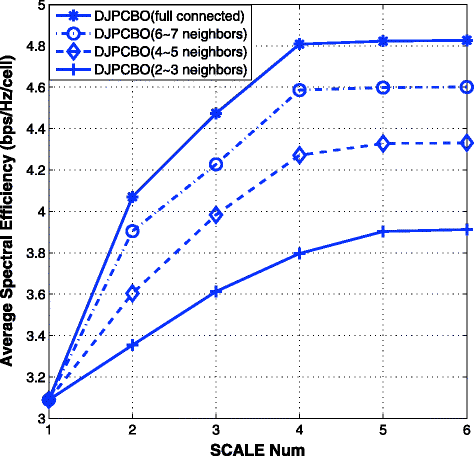

  

  System performance with the increasing SCALE iteration.

  Figure 8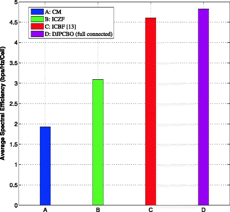

  

  Comparison of average spectral efficiency between different strategies.

• 2) Intra-cell zero-forcing (ICZF) beamforming: the set of beams is designed so as to eliminate intra-cell interference, i.e.,

  $${} {{\mathbf{w}}_{i,j}}\left(q \right)={\delta_{i,j}}\left(q \right)\sqrt {\frac{{{P_{\max }}}}{{{K_{i}}Q}}} {\left({\sum\limits_{l}^{{K_{i}}} {{{\mathbf{h}}_{i,i,l}}\left(q \right){\mathbf{h}}_{i,i,l}^{H}\left(q \right)}} \right)^{- 1}}{{\mathbf{h}}_{i,i,j}}\left(q \right) $$

As shown in Figure 8, the CM strategy is not a good choice in multi-cell multi-antenna scenario, for the poor average network capacity resulted from ignoring the co-channel interference. Comparatively, ICZF scheme is better than the CM strategy by utilizing orthogonal beamforming vectors in single cell. However, its capability is still limited. Due to that the proposed DJPCBO takes the inter-cell interference into account, much gain can be achieved from the coordination among HeNBs. Thus, it validates that the proposed DJPCBO algorithm outperforms the two existing benchmark techniques a lot. Moreover, we also compare the DJPCBO algorithm with the cooperating strategy ICBF [13], under the same initial beamforming state, and we have found DJPCBO is better than ICBF algorithm. It is worth noting that the initial beamforming state will affect the algorithm performance due to the nature of SCALE approximation [22], i.e., a good initial state presents an excellent gain. We consequently choose the ICZF strategy as the initial state in the simulation.

Furthermore, Figure 9 presents the spectral efficiency of cells served by different HeNBs respectively. When compared to the CM and ICZF schemes, most cells’ performances are promoted through using the proposed DJPCBO algorithm. Moveover, from this figure, each HeNB’s spectral efficiency is slightly better than the ICBF which does not take the cooperation graph into consideration. However, a few of them are even worse. That is because the quality of service (QoS) has not been taken into account. In our future works, the QoS guarantee will be considered as an additional constraint.

Figure 9

Spectral efficiency performance for HeNBs 1 to 9.

5 Conclusions

In this paper, the NP-hard WSRMax problem in multiple input single output (MISO) HeNB network is studied. With an ameliorated max-min multi-cell uplink-downlink throughput duality, a distributed algorithm based on two loops is proposed to solve this problem. In Loop1, we apply DLPDS algorithm to solve the virtual uplink programming. Furthermore, we propose a new iteration scheme to optimize the virtual noise problem with separable structure in Loop2. Numerical results show the two loops can converge to a stable state, and the network performance is dramatically improved with the coordinations among HeNBs. Thus, it can be seen that multi-cell uplink-downlink throughput duality is a powerful tool to solve WSRMax problem. In the future, we will apply this tool into multi-input multi-output scenarios and take the QoS into consideration.

6 Appendix A: proof of Lemma 1

The proof of Lemma 1 is similar with the proof in [18], and we provide it here for completeness reason. The primal problem (1) can be reformulated into an equivalent form:

$${} \left\{ {\fontsize{7.6pt}{9.6pt}\selectfont{\begin{aligned} &\mathop {\max }\limits_{{\mathbf{p}}, {\mathbf{w}}} {{\sum\nolimits}_{i}^{N}} {{{\sum\nolimits}_{q}^{Q}} {{\sum\nolimits}_{j}^{{K_{i}}} {\left\{ {{\alpha_{i,j}}\left(q \right){{\log }_{2}}\left[ {\gamma_{i,j}}\left(q \right) \right] + {\beta_{i,j}}\left(q \right)} \right\}}} } \\ & s.t\;\;\;{C_{1}}:\;{\gamma_{i,j}}\left(q \right) \le \frac{{{p_{i,j}}\left(q \right){{\left| {{\mathbf{h}}_{i,i,j}^{H}\left(q \right){{\mathbf{w}}_{i,j}}\left(q \right)} \right|}^{2}}}}{{{\sigma_{n}^{2}} + {\sum\nolimits}_{m = 1}^{{N_{i}}} {{\sum\nolimits}_{\left({m,n} \right) \ne \left({i,j} \right)}^{{K_{m}}} {{p_{m,n}}\left(q \right){{\left| {{\mathbf{h}}_{m,i,j}^{H}\left(q \right){{\mathbf{w}}_{m,n}}\left(q \right)} \right|}^{2}}}} }}\\ & {C_{2}}:\;{{\sum\nolimits}_{q}^{Q}} {{\sum\nolimits}_{j}^{{K_{i}}} {{p_{i,j}}\left(q \right)}} \le {P_{\max }}\\ &{C_{3}}:\;{p_{i,j}}\left(q \right) \ge 0\;\;\;\;\;\;\;\;\;\;\forall i,i = 1,\ldots N;\forall q,q = 1,\ldots Q;\forall j,j = 1,\ldots K, \end{aligned}}} \right. $$

((24))

where γ _i,j (q) is the lower bound of downlink SINR. By rearranging the C ₁ constraint in (24), the Lagrangian function is given by:

$${} {\fontsize{9.2}{6}\begin{aligned} &L\left({ {\mathbf{\gamma }}, {\mathbf{p}}, {\mathbf{w}}, {{{\mathbf{\lambda }}_{\mathbf{1}}}}, {{{\mathbf{\lambda }}_{\mathbf{2}}}}, {{{\mathbf{\lambda }}_{\mathbf{3}}}}} \right)\\ &= {{\sum\nolimits}_{i}^{N}} {{{\sum\nolimits}_{q}^{Q}} {{\sum\nolimits}_{j}^{{K_{i}}} {\left\{ {\alpha_{i,j}\left(q \right){{\log }_{2}}\left[ {{\gamma_{i,j}}\left(q \right)} \right]+ {\beta_{i,j}}\left(q \right)} \right\}}} } \\ &\hspace*{6pt}- {{\sum\nolimits}_{i}^{N}} {{{\sum\nolimits}_{q}^{Q}} {{\sum\nolimits}_{j}^{{K_{i}}} {{\lambda_{1,i,j}}\left(q \right)\!\left(\!\vphantom{\frac{{{p_{i,j}}\left(q \right){{\left| {{\mathbf{h}}_{i,i,j}^{H}\left(q \right) {{\mathbf{w}}_{i,j}}\left(q \right)} \right|}^{2}}}}{{{{\gamma }_{i,j}}\left(q \right)}} + {\sigma_{n}^{2}}} {{{{\sum\nolimits}_{l \ne j}^{{K_{i}}} {{p_{i,l}}\left(q \right)\left| {{\mathbf{h}}_{i,i,j}^{H}\left(q \right) {{\mathbf{w}}_{i,l}}\left(q \right)} \right|} }^{2}}} \right.}}} \\ &\hspace*{6pt}+\left. \sum\limits_{m \ne i}^{{N_{i}}} {\sum\limits_{n}^{{K_{m}}} {{p_{m,n}}\left(q \right){{\left| {{\mathbf{h}}_{m,i,j}^{H}\left(q \right) {{\mathbf{w}}_{m,n}}\left(q \right)} \right|}^{2}}}}\right. \\ &\hspace*{6pt}-\left. \frac{{{p_{i,j}}\left(q \right){{\left| {{\mathbf{h}}_{i,i,j}^{H}\left(q \right) {{\mathbf{w}}_{i,j}}\left(q \right)} \right|}^{2}}}}{{{{\gamma }_{i,j}}\left(q \right)}} + {\sigma_{n}^{2}} \right)\\ &\hspace*{6pt}- {{\sum\nolimits}_{i}^{N}} {{\lambda_{2,i}}\left({{{\sum\nolimits}_{q}^{Q}} {{\sum\nolimits}_{j}^{{K_{i}}} {{p_{i,j}}\left(q \right)}} - {P_{\max }}} \right)} \\&\hspace*{6pt}+ {{\sum\nolimits}_{i}^{N}} {{{\sum\nolimits}_{q}^{Q}} {{\sum\nolimits}_{j}^{{K_{i}}} {{\lambda_{3,i,j}}\left(q \right){p_{i,j}}\left(q \right)}} }, \end{aligned}} $$

((25))

where {λ ₁ },{λ ₂ },{λ ₃ } are the Lagrangian multipliers associating with constraint C ₁,C ₂,C ₃, respectively. The following equality can be obtained by rearranging (25):

$$ \begin{aligned} &L\left({{\gamma}, {\mathbf{p}}, {\mathbf{w}}, {{\lambda}}_{\mathbf{1}}}, {{\lambda}_{\mathbf{2}}}, {\lambda}_{\mathbf{3}} \right) \\ &= {\sum\limits_{i}^{N}} {{\sum\limits_{q}^{Q}} {\sum\limits_{j}^{{K_{i}}} {\left\{ {\alpha_{i,j}\left(q \right){{\log }_{2}}\left[ {{\gamma_{i,j}}\left(q \right)} \right]+ {\beta_{i,j}}\left(q \right)} \right\}}} } \\ &\hspace*{6pt} - {\sum\limits_{i}^{N}} {{\sum\limits_{q}^{Q}} {\sum\limits_{j}^{{K_{i}}} {{\lambda_{1,i,j}}\left(q \right)}} } {\sigma_{n}^{2}} + {{\sum\nolimits}_{i}^{N}} {{\lambda_{2,i}}{P_{\max }}}\\ &\hspace*{6pt}+ {{\sum\nolimits}_{i}^{N}} {{\sum\nolimits}_{q}^{Q}} {\sum\nolimits}_{j}^{{K_{i}}} {p_{i,j}}\left(q\right) \left\{{{\lambda_{1,i,j}}\left(q\right){{\left| {{\mathbf{w}}_{i,j}^{H}\left(q \right){{\mathbf{h}}_{i,i,j}}\left(q \right)} \right|}^{2}}} \right. \\ &\hspace*{6pt}- {\sum\nolimits}_{m}^{{N_{i}}} {{\sum\nolimits}_{n}^{{K_{m}}} {{\lambda_{1,m,n}}\left(q \right){{\left| {{\mathbf{w}}_{i,j}^{H}\left(q \right){{\mathbf{h}}_{i,m,n}}\left(q \right)} \right|}^{2}}}} \\ &\hspace*{6pt}+ \frac{{{\lambda_{1,i,j}}\left(q \right){{\left| {{\mathbf{w}}_{i,j}^{H}\left(q \right){{\mathbf{h}}_{i,i,j}}\left(q \right)} \right|}^{2}}}}{{{\gamma_{i,j}}\left(q \right)}} \left.{\vphantom{\frac{0}{0}}} { - {\lambda_{2,i}} + {\lambda_{3,i,j}}\left(q \right)} \right\}. \end{aligned} $$

((26))

The corresponding dual objective problem can be expressed as:

$$ g\left({ {{\lambda}_{1}}}, {{\lambda}_{2}}, {{{\lambda}_{3}}} \right) = \mathop {\max }\limits_{{\gamma}, {\mathbf{p}},\left\{{\mathbf{w}} \right\}} L\left({{\gamma}, {\mathbf{p}}, {\mathbf{w}}, {{\lambda}_{1}}}, {{\lambda}_{2}}, {{\lambda}_{3}} \right).\hspace*{50pt} $$

((27))

According to the KKT condition, $\frac {{\partial L}}{{\partial {p_{i,j}}\left (q \right)}} = 0$ at optimum and the fact λ _3,i,j (q)≥0, the underlying inequality is hold:

$${} {\fontsize{7.8pt}{9.6pt}\selectfont{\begin{aligned} &{\gamma_{i,j}}\left(q \right)\\ &\ge \frac{{{p_{i,j}}\left(q \right){{\left| {{\mathbf{h}}_{i,i,j}^{H}\left(q \right) {{\mathbf{w}}_{i,j}}\left(q \right)} \right|}^{2}}}}{{{\lambda_{2,i}} + \sum\limits_{m}^{{N_{i}}} {\sum\limits_{n}^{{K_{m}}} {{\lambda_{1,m,n}}\left(q \right){{\left| {{\mathbf{w}}_{i,j}^{H}\left(q \right){{\mathbf{h}}_{i,m,n}}\left(q \right)} \right|}^{2}}}} - {\lambda_{1,i,j}}\left(q \right){{\left| {{\mathbf{w}}_{i,j}^{H}\left(q \right){{\mathbf{h}}_{i,i,j}}\left(q \right)} \right|}^{2}}}}\\ &= \frac{{{{\lambda }_{{1},i,j}}\left(q \right){{\left| {{\mathbf{w}}_{i,j}^{H}\left(q \right){{\mathbf{h}}_{i,i,j}}\left(q \right)} \right|}^{2}}}}{{{\lambda_{2,i}} + {\sum\nolimits}_{m=1}^{{N_{i}}} {{\sum\nolimits}_{(m,n)\neq(i,j)}^{{K_{m}}} {{\lambda_{1,m,n}}\left(q \right){{\left| {{\mathbf{w}}_{i,j}^{H}\left(q \right){{\mathbf{h}}_{i,m,n}}\left(q \right)} \right|}^{2}}}} }}. \end{aligned}}} $$

((28))

With (27) and (28), the dual problem can be explicitly expressed as:

$${} \left\{ {\fontsize{8.2pt}{9.6pt}\selectfont{\begin{aligned} &\mathop {\min }\limits_{{{{\mathbf{\lambda }}_{\mathbf{1}}}}, {{{\mathbf{\lambda }}_{\mathbf{2}}}}} \mathop {\max }\limits_{{\mathbf{w}}, {\mathbf{\gamma }}} {{\sum\nolimits}_{i}^{N}} {{{\sum\nolimits}_{q}^{Q}} {{\sum\nolimits}_{j}^{{K_{i}}} {\left\{ {\alpha_{i,j}\left(q \right){{\log }_{2}}\left[ {{\gamma_{i,j}}\left(q \right)} \right]+ {\beta_{i,j}}\left(q \right)} \right\}}} } \\ &- {{\sum\nolimits}_{i}^{N}} {{{\sum\nolimits}_{q}^{Q}} {{\sum\nolimits}_{j}^{{K_{i}}} {{\lambda_{1,i,j}}\left(q \right)}} } {\sigma_{n}^{2}}+ {{\sum\nolimits}_{i}^{N}} {{\lambda_{2,i}}{P_{\max }}} \\ &s.t{C_{1}}:{\gamma_{i,j}}\left(q \right) \ge \frac{{{{\lambda }_{{1},i,j}}\left(q \right){{\left| {{\mathbf{w}}_{i,j}^{H}\left(q \right){{\mathbf{h}}_{i,i,j}}\left(q \right)} \right|}^{2}}}}{{{\lambda_{2,i}} + \sum\limits_{m=1}^{{N_{i}}} {\sum\limits_{(m,n)\neq(i,j)}^{{K_{m}}} {{\lambda_{1,m,n}}\left(q \right){{\left| {{\mathbf{w}}_{i,j}^{H}\left(q \right){{\mathbf{h}}_{i,m,n}}\left(q \right)} \right|}^{2}}}} }}\\ &{C_{2}}:{\lambda_{1,i,j}}\left(q \right) \ge 0\;\;\;\;\;\;\;\;\;\forall i,i = 1,\ldots N;\forall q,j = 1,\ldots Q;\forall j,j = 1,\ldots K\\ &{C_{3}}:{\lambda_{2,i}} \ge 0\;\;\;\;\;\;\;\;\;\;\;\;\;\;\;\;\forall i,i = 1,\ldots N. \end{aligned}}} \right. $$

((29))

The term ${{\sum \nolimits }_{i}^{N}} {{{\sum \nolimits }_{q}^{Q}} {{\sum \nolimits }_{j}^{{K_{i}}} {{\lambda _{1,i,j}}\left (q \right)}} } {\sigma _{n}^{2}}$ of the objective function in (29) can be moved into the constraint set by introducing a Lagrange multiplier χ, and the equivalent problem is:

$${} \left\{ {\fontsize{7.4pt}{9.6pt}\selectfont{\begin{aligned} &\mathop {\max }\limits_{\chi} \!\mathop {\min }\limits_{{{{\mathbf{\lambda }}_{\mathbf{1}}}}, {{{\mathbf{\lambda }}_{\mathbf{2}}}}} \!\mathop {\max }\limits_{{\mathbf{w}}, {\mathbf{\gamma }}} {\sum\limits_{i}^{N}} {{\sum\limits_{q}^{Q}} {\sum\limits_{j}^{{K_{i}}} {\left\{ {\alpha_{i,j}\left(q \right){{\log }_{2}}\left[ {{\gamma_{i,j}}\left(q \right)} \right]\,+\, {\beta_{i,j}}\left(q \right)} \right\}}} } \,+\, {{\sum\nolimits}_{i}^{N}} {{\lambda_{2,i}}{P_{\max }}}\! - \!\chi \\ &s.t\hspace{8pt}{C_{1}}:{\gamma_{i,j}}\left(q \right) \ge \frac{{{{\lambda }_{{1},i,j}}\left(q \right){{\left| {{\mathbf{w}}_{i,j}^{H}\left(q \right){{\mathbf{h}}_{i,i,j}}\left(q \right)} \right|}^{2}}}}{{{\lambda_{2,i}} + {\sum\nolimits}_{m=1}^{{N_{i}}} {{\sum\nolimits}_{(m,n)\neq(i,j)}^{{K_{m}}} {{\lambda_{1,m,n}}\left(q \right){{\left| {{\mathbf{w}}_{i,j}^{H}\left(q \right){{\mathbf{h}}_{i,m,n}}\left(q \right)} \right|}^{2}}}} }}\\ &{C_{2}}:{\lambda_{1,i,j}}\left(q \right) \ge 0\;\;\;\;\;\;\;\;\;\forall i,i = 1,\ldots N;\forall q,j = 1,\ldots Q;\forall j,j = 1,\ldots K\\ &{C_{3}}:{\lambda_{2,i}} \ge 0\;\;\;\;\;\;\;\;\;\;\;\;\;\;\;\;\forall i,i = 1,\ldots N\\ &{C_{4}}:{{\sum\nolimits}_{i}^{N}} {{{\sum\nolimits}_{q}^{Q}} {{\sum\nolimits}_{j}^{{K_{i}}} {{\lambda_{1,i,j}}\left(q \right)}} } {\sigma_{n}^{2}} \le \chi. \end{aligned}}} \right. $$

((30))

A further transformation rule with χ ^′, ${{\bar \lambda }_{1,i,j}}\left (q \right)$, and ${{\bar \lambda }_{2,i}}$ is presented as follows:

$$ \left\{ \begin{aligned} &\chi = \chi '{\sigma_{n}^{2}}{\sum\nolimits}_{i = 1}^{N} {{P_{\max }}}, \\ &{\lambda_{1,i,j}}\left(q \right) = \chi '{{\bar \lambda }_{1,i,j}}\left(q \right),\\ &{\lambda_{2,i}} = \chi '{{\bar \lambda }_{2,i}}, \end{aligned} \right. $$

((31))

and the equivalent dual problem can be stated as

$${} \left\{ {\fontsize{7.6pt}{9.6pt}\selectfont{\begin{aligned} &\mathop {\max }\limits_{\chi '} \mathop {\min }\limits_{{{{\bar{\mathbf{ \lambda }}}_{\mathbf{1}}}}, {{{\bar{\mathbf{ \lambda }}}_{\mathbf{2}}}}} \mathop {\max }\limits_{{\mathbf{w}}, {\mathbf{\gamma }} } {\sum\limits_{i}^{N}} {{\sum\limits_{q}^{Q}} {\sum\limits_{j}^{{K_{i}}} {\left\{ {\alpha_{i,j}\left(q \right){{\log }_{2}}\left[ {{\gamma_{i,j}}\left(q \right)} \right]+ {\beta_{i,j}}\left(q \right)} \right\}}} } \\ &+ \chi '\left\{ {{\sum\limits_{i}^{N}} {{{\bar \lambda }_{2,i}}{P_{\max }}} - {\sigma_{n}^{2}}{\sum\limits_{i}^{N}} {{P_{\max }}}} \right\}\\ &s.t\;\;{C_{1}}:{\gamma_{i,j}}\left(q \right) \ge \frac{{{{\bar{\lambda} }_{{1},i,j}}\left(q \right){{\left| {{\mathbf{w}}_{i,j}^{H}\left(q \right){{\mathbf{h}}_{i,i,j}}\left(q \right)} \right|}^{2}}}}{{{\bar{\lambda}_{2,i}} + {\sum\nolimits}_{m=1}^{{N_{i}}} {{\sum\nolimits}_{(m,n)\neq(i,j)}^{{K_{m}}} {{\bar{\lambda}_{1,m,n}}\left(q \right){{\left| {{\mathbf{w}}_{i,j}^{H}\left(q \right){{\mathbf{h}}_{i,m,n}}\left(q \right)} \right|}^{2}}}} }}\\ &{C_{2}}:{{\bar \lambda }_{1,i,j}}\left(q \right) \ge 0\;\;\;\;\;\;\;\;\;\forall i,i = 1,\ldots N;\forall q,j = 1,\ldots Q;\forall j,j = 1,\ldots K\\ &{C_{3}}:{{\bar \lambda }_{2,i}} \ge 0\forall i,i = 1,\ldots N\\ &{C_{4}}:{{\sum\nolimits}_{i}^{N}} {{{\sum\nolimits}_{q}^{Q}} {{\sum\nolimits}_{j}^{{K_{i}}} {{{\bar \lambda }_{1,i,j}}}} } \left(q \right) \le {{\sum\nolimits}_{i}^{N}} {{P_{\max }}}. \end{aligned}}} \right. $$

((32))

χ ^′ can be considered as a dual multiplier of the constraint ${\sum \limits _{i}^{N}} {{{\bar \lambda }_{2,i}}{P_{\max }}\! -\! {\sigma _{n}^{2}}{\sum \limits _{i}^{N}} {{P_{\max }}}} \le 0$, and for other fixed variables, optimization over ${\bar \lambda _{2,i}}$ is a convex problem that guarantees strong duality. By changing (32) as primal problem over ${\bar \lambda _{2,i}}$ with a constraint, the corresponding equivalent dual problem is:

$${} \left\{ {\fontsize{7.6pt}{9.6pt}\selectfont{\begin{aligned} &\mathop {\min }\limits_{{{{\bar{\mathbf{ \lambda }}}_{\mathbf{1}}}}, {{{\bar{\mathbf{ \lambda }}}_{\mathbf{2}}}}} \mathop {\max }\limits_{{\mathbf{w}}, {\mathbf{\gamma }}} {{\sum\nolimits}_{i}^{N}} {{{\sum\nolimits}_{q}^{Q}} {{\sum\nolimits}_{j}^{{K_{i}}} {\left\{ {\alpha_{i,j}\left(q \right){{\log }_{2}}\left[ {{\gamma_{i,j}}\left(q \right)} \right]+ {\beta_{i,j}}\left(q \right)} \right\}}} } \\ &s.t\;\;{C_{1}}:{\gamma_{i,j}}\left(q \right) \ge \frac{{{{\bar{\lambda} }_{{1},i,j}}\left(q \right){{\left| {{\mathbf{w}}_{i,j}^{H}\left(q \right){{\mathbf{h}}_{i,i,j}}\left(q \right)} \right|}^{2}}}}{{{\bar{\lambda}_{2,i}} + {\sum\nolimits}_{m=1}^{{N_{i}}} {{\sum\nolimits}_{(m,n)\neq(i,j)}^{{K_{m}}} {{\bar{\lambda}_{1,m,n}}\left(q \right){{\left| {{\mathbf{w}}_{i,j}^{H}\left(q \right){{\mathbf{h}}_{i,m,n}}\left(q \right)} \right|}^{2}}}} }}\\ &\;\;\;\;\;{C_{2}}:{{\bar \lambda }_{1,i,j}}\left(q \right) \ge 0\;\;\;\;\;\;\;\;\;\forall i,i = 1,\ldots N;\forall q,q = 1,\ldots Q;\forall j,j = 1,\ldots K\\ &\;\;\;\;\;{C_{3}}:{{\bar \lambda }_{2,i}} \ge 0\forall i,i = 1,\ldots N\\ &\;\;\;\;\;{C_{4}}:{{\sum\nolimits}_{i}^{N}} {{{\sum\nolimits}_{q}^{Q}} {{\sum\nolimits}_{j}^{{K_{i}}} {{{\bar \lambda }_{1,i,j}}\left(q \right)}} } \le {{\sum\nolimits}_{i}^{N}} {{P_{\max }}} \\ &\;\;\;\;\;{C_{5}}:{{\sum\nolimits}_{i}^{N}} {{{\bar \lambda }_{2,i}}{P_{\max }}} \le {\sigma_{n}^{2}}{{\sum\nolimits}_{i}^{N}} {{P_{\max }}}. \end{aligned}}} \right. $$

((33))

Since the optimization is met with equality for fixed ${\gamma _{i,j}}\left (q \right),{\bar \lambda _{2,i}},{{\mathbf {w}}_{i,j}}\left (q \right)$, reversal of the SINR constraint and the reversal of the C ₁ minimization as a maximization over ${\bar \lambda _{1,i,j}}\left (q \right)$ do not change the optimization problem. Thus, the modified dual problem can be stated as:

$${} \left\{ {\fontsize{7.6pt}{9.6pt}\selectfont{\begin{aligned} &\mathop {\min }\limits_{{{{\bar{\mathbf{ \lambda }}}_{\mathbf{2}}}}} \mathop {\max }\limits_{{{{\bar{\mathbf{ \lambda }}}_{\mathbf{1}}}}, {\mathbf{w}}, {\mathbf{\gamma }}} {{\sum\nolimits}_{i}^{N}} {{{\sum\nolimits}_{q}^{Q}} {{\sum\nolimits}_{j}^{{K_{i}}} {\left\{ {\alpha_{i,j}\left(q \right){{\log }_{2}}\left[ {{\gamma_{i,j}}\left(q \right)} \right]+ {\beta_{i,j}}\left(q \right)} \right\}}} } \\ &s.t\;\;{C_{1}}:{\gamma_{i,j}}\left(q \right) \ge \frac{{{{\bar{\lambda} }_{{1},i,j}}\left(q \right){{\left| {{\mathbf{w}}_{i,j}^{H}\left(q \right){{\mathbf{h}}_{i,i,j}}\left(q \right)} \right|}^{2}}}}{{{\bar{\lambda}_{2,i}} + {\sum\nolimits}_{m=1}^{{N_{i}}} {{\sum\nolimits}_{(m,n)\neq(i,j)}^{{K_{m}}} {{\bar{\lambda}_{1,m,n}}\left(q \right){{\left| {{\mathbf{w}}_{i,j}^{H}\left(q \right){{\mathbf{h}}_{i,m,n}}\left(q \right)} \right|}^{2}}}} }}\\ &{C_{2}}:{{\bar \lambda }_{1,i,j}}\left(q \right) \ge 0\;\;\;\;\;\;\;\;\;\forall i,i = 1,\ldots N;\forall j,j = 1,\ldots K\\ &{C_{3}}:{{\bar \lambda }_{2,i}} \ge 0\;\;\;\;\;\;\;\;\;\;\;\forall i,i = 1,\ldots N\\ &{C_{4}}:{{\sum\nolimits}_{i}^{N}} {{{\sum\nolimits}_{q}^{Q}} {{\sum\nolimits}_{j}^{{K_{i}}} {{{\bar \lambda }_{1,i,j}}}} } \left(q \right) \le {{\sum\nolimits}_{i}^{N}} {{P_{\max }}} \\ &{C_{5}}:{{\sum\nolimits}_{i}^{N}} {{{\bar \lambda }_{2,i}}{P_{\max }}} \le {\sigma_{n}^{2}}{{\sum\nolimits}_{i}^{N}} {{P_{\max }}}. \end{aligned}}} \right. $$

((34))

Replacing γ _i,j (q) with the right term of the inequality constraint in (34) completes the proof.

Moreover, as the virtual uplink sum power {λ _1,i,j } is upper bounded by real downlink power P _max, and according to the duality theory [26], the optimal value of the dual objective function is lower bounded by the maximum value of the primal maximization problem (4). The strong duality is analyzed in [18] and is further applied in [19] successfully.

7 Appendix B: proof of Lemma 2

We substitute g _i (·) into (16a) with z _i =y and obtain:

$$ \begin{array}{l} z_{i}^{k + 1} = \mathop {\arg \max }\limits_{{z_{i}} \ge 0} \mathop {\inf }\limits_{{{\bar \lambda }_{2,i}\in {{\mathbf{\chi }}_{i}}}} \left\{ K\left({{{\bar \lambda }_{2,i}},{z_{i}}} \right) \right\}, \end{array} $$

((35))

where $K\left ({{{\bar \lambda }_{2,i}},{z_{i}}} \right):R \times R \rightarrow R$ is defined as:

$${} {\fontsize{8.8pt}{9.6pt}\selectfont{\begin{aligned} &K\left({{{\bar \lambda }_{2,i}},{z_{i}}} \right)\\ &= {f_{i}}\left({{{\bar \lambda }_{2,i}}} \right) + {z_{i}}{c_{i}}\left({{{\bar \lambda }_{2,i}}} \right) - \sum\limits_{l \in S\left(i \right)} {\left[ {\lambda_{il}^{k}\left({{z_{i}} - {z_{l}^{k}}} \right) + \frac{\rho }{2}{{\left\| {{z_{i}} - {z_{l}^{k}}} \right\|}^{2}}} \right]} \\ &- \sum\limits_{l \in P\left(i \right)} {\left[ {\lambda_{li}^{k}\left({z_{l}^{k + 1} - {z_{i}}} \right) + \frac{\rho }{2}{{\left\| {z_{l}^{k + 1} - {z_{i}}} \right\|}^{2}}} \right]} \quad\!\! \text{for}\; {{\bar \lambda }_{2,i}\in {{\mathbf{\chi }}_{i}}}, z_{i}\ge 0. \end{aligned}}} $$

((36))

If the solution set is non-empty and bounded, then the function f _i (·), c _i (·) and the set χ _i have no direction of recession in the sense of ([27], p. 61 and p. 69). It can be deduced that the convex function K(·,z _i ) has no direction of recession of for any z _i ≥0, while the convex function $-K\left ({{{\bar \lambda }_{2,i}},\cdot } \right)$ has no direction of recession for any ${{\bar \lambda }_{2,i}\in {{\mathbf {\chi }}_{i}}}$. According to the theorems 37.3 and 37.6 in [27], the saddle point $({\bar \lambda }_{2,i},z_{i}) \in {\mathbf {\chi }}_{i} \times \{z_{i}|z_{i} \geq 0\}$ exists:

$$ \mathop {\sup }\limits_{{z_{i}} \ge 0} \mathop {\inf }\limits_{{{\bar \lambda }_{2,i}} \in {\chi_{i}}} \left[ {K\left({{{\bar \lambda }_{2,i}},{z_{i}}} \right)} \right] = \mathop {\inf }\limits_{{{\bar \lambda }_{2,i}} \in {\chi_{i}}} \mathop {\sup }\limits_{{z_{i}} \ge 0} \left[ {K\left({{{\bar \lambda }_{2,i}},{z_{i}}} \right)} \right]. $$

((37))

Moreover, since the value of the saddle point will not change by adding constant terms, we could obtain:

$${} \begin{aligned} &\mathop {\max }\limits_{{z_{i}} \ge 0} \mathop {\min }\limits_{{{\bar \lambda }_{2,i}\in {{\mathbf{\chi }}_{i}}}} \left\{ K\left({{{\bar \lambda }_{2,i}},{z_{i}}} \right) - \sum\limits_{l \in S\left(i \right)} {\left[ {\lambda_{il}^{k}{z_{l}^{k}} - \frac{\rho }{2}{{\left({{z_{l}^{k}}} \right)}^{2}}} \right]}\right. \\&\qquad\qquad\quad+\left. \sum\limits_{l \in P\left(i \right)} {\left[ {\lambda_{li}^{k}z_{l}^{k + 1} + \frac{\rho }{2}{{\left({z_{l}^{k + 1}} \right)}^{2}}} \right]} \right\}\\ &= \mathop {\min }\limits_{{{\bar \lambda }_{2,i}\in {{\mathbf{\chi }}_{i}}}} \mathop {\max }\limits_{{z_{i}} \ge 0} \left\{ K\left({{{\bar \lambda }_{2,i}},{z_{i}}} \right) - \sum\limits_{l \in S\left(i \right)} {\left[ {\lambda_{il}^{k}{z_{l}^{k}} - \frac{\rho }{2}{{\left({{z_{l}^{k}}} \right)}^{2}}} \right]} \right. \\&\qquad\qquad\quad+\left.\sum\limits_{l \in P\left(i \right)} {\left[ {\lambda_{li}^{k}z_{l}^{k + 1} + \frac{\rho }{2}{{\left({z_{l}^{k + 1}} \right)}^{2}}} \right]} \right\}. \end{aligned} $$

((38))

Consequently, for fixed any ${\bar \lambda }_{2,i}$, the maximum on the right side of (41) is uniquely attained by:

$$ {z_{i}} = \max \left\{ {0,\frac{1}{{\rho \left({{S_{i}} + {P_{i}}} \right)}}\left[ {{c_{i}}\left({{{\bar \lambda }_{2,i}}} \right) + A_{i} + B_{i}} \right]} \right\}. $$

((39))

We substitute (39) into the right side of (38) to eliminate z _i . Due to (39) is a piecewise function, two cases need to be considered respectively:

Case 1: if z _i =0, we obtain:

$$ \bar \lambda_{2,i}^{k + 1} = \mathop {\arg \min }\limits_{{{\bar \lambda }_{2,i}} \in {\chi_{i}}} {f_{i}}\left({{{\bar \lambda }_{2,i}}} \right). $$

((40))

Case 2: if $z_{i}=\left [ {{c_{i}}\left ({{{\bar \lambda }_{2,i}}} \right) + A_{i} + B_{i}}\right ]/\left [{{\rho \left ({{S_{i}} + {P_{i}}} \right)}}\right ]$, we obtain:

$${} {\fontsize{7.4pt}{9.6pt}\selectfont{\begin{aligned} &K\left({{{\bar \lambda }_{2,i}},{z_{i}}} \right) - \sum\limits_{l \in S\left(i \right)} {\left[ {\lambda_{il}^{k}{z_{l}^{k}} - \frac{\rho }{2}{{\left({{z_{l}^{k}}} \right)}^{2}}} \right]} + \sum\limits_{l \in P\left(i \right)} {\left[ {\lambda_{li}^{k}z_{l}^{k + 1} + \frac{\rho }{2}{{\left({z_{l}^{k + 1}} \right)}^{2}}} \right]} \\ &= {f_{i}}\left({{{\bar \lambda }_{2,i}}} \right) + \left\{ \sum\limits_{l \in S\left(i \right)} \left[ \frac{1}{{{P_{i}} + {S_{i}}}}{z_{i}}{c_{i}}\left({{{\bar \lambda }_{2,i}}} \right) - \lambda_{il}^{k}{z_{i}} - \frac{\rho }{2}{{\left({{z_{i}} - {z_{l}^{k}}} \right)}^{2}} + \frac{\rho }{2}{{\left({{z_{l}^{k}}} \right)}^{2}} \right] \right\}_{1}\\ &\quad+ {\left\{ {\sum\limits_{l \in P\left(i \right)} {\left[ {\frac{1}{{{P_{i}} + {S_{i}}}}{z_{i}}{c_{i}}\left({{{\bar \lambda }_{2,i}}} \right) + \lambda_{li}^{k}{z_{i}} - \frac{\rho }{2}{{\left({z_{l}^{k + 1} - {z_{i}}} \right)}^{2}} + \frac{\rho }{2}{{\left({z_{l}^{k + 1}} \right)}^{2}}} \right]}} \right\}_{2}}. \end{aligned}}} $$

((41))

Next, we give the first priority to {·}₁:

$${} \begin{aligned} &{\left\{ \cdot \right\}_{1}}\\ &= - \sum\limits_{l \in S\left(i \right)} {\left\{ {\frac{\rho }{2}{z_{i}^{2}} + {z_{i}}\left[ {\lambda_{il}^{k} - \rho {z_{l}^{k}} - \frac{{{c_{i}}\left({{{\bar \lambda }_{2,i}}} \right)}}{{{P_{i}} + {S_{i}}}}} \right]} \right\}} \\ &= \frac{1}{{2\rho {{\left({{P_{i}} + {S_{i}}} \right)}^{2}}}}\left\{ {S_{i}}{{\left[ {{c_{i}}\left({{{\bar \lambda }_{2,i}}} \right)} \right]}^{2}} + 2\left({{P_{i}} + {S_{i}}} \right)A_{i}{c_{i}}\left({{{\bar \lambda }_{2,i}}} \right)\right.\\ & \qquad\qquad\qquad\quad + \left. 2\left({{P_{i}} \,+\, {S_{i}}} \right)\left({A_{i} \,+\, B_{i}} \right)A_{i} \,-\, {S_{i}}{{\left({A_{i} \,+\, B_{i}} \right)}^{2}} \vphantom{{S_{i}}{{\left[ {{c_{i}}\left({{{\bar \lambda }_{2,i}}} \right)} \right]}^{2}} + 2\left({{P_{i}} + {S_{i}}} \right)A_{i}{c_{i}}\left({{{\bar \lambda }_{2,i}}} \right)}\!\right\}. \end{aligned} $$

((42))

Similar to {·}₁, {·}₂ can be represented as:

$${} \begin{aligned} &{\left\{ \cdot \right\}_{2}}\\ &= \sum\limits_{l \in P\left(i \right)} {\left\{ {-\frac{\rho }{2}{z_{i}^{2}} + {z_{i}}\left[ {\lambda_{li}^{k} +\rho z_{l}^{k+1} + \frac{{{c_{i}}\left({{{\bar \lambda }_{2,i}}} \right)}}{{{P_{i}} + {S_{i}}}}} \right]} \right\}}\\ &= \frac{1}{{2\rho {{\left({{P_{i}} + {S_{i}}} \right)}^{2}}}}\left\{ {P_{i}}{{\left[ {{c_{i}}\left({{{\bar \lambda }_{2,i}}} \right)} \right]}^{2}}\!\! + 2\left({{P_{i}} + {S_{i}}} \right)B_{i}{c_{i}}\left({{{\bar \lambda }_{2,i}}} \right)\right.\\ & \qquad\qquad\qquad\quad+ \left. 2\left({{P_{i}} + {S_{i}}} \right)\left({A_{i} + B_{i}} \right)B_{i}\! -\! {P_{i}}{{\left({A_{i}\! +\! B_{i}} \right)}^{2}} \vphantom{{P_{i}}{{\left[ {{c_{i}}\left({{{\bar \lambda }_{2,i}}} \right)} \right]}^{2}}\!\! + 2\left({{P_{i}} + {S_{i}}} \right)B_{i}{c_{i}}\left({{{\bar \lambda }_{2,i}}} \right)}\right\}\!. \end{aligned} $$

((43))

We substitute (42) (43) into (38) and obtain:

$${} {\fontsize{8.8pt}{9.6pt}\selectfont{\begin{aligned} \bar \lambda_{2,i}^{k + 1} = \mathop {\arg \min }\limits_{{{\bar \lambda }_{2,i}} \ge 0} \left\{ \,{{f_{i}}\left({{{\bar \lambda }_{2,i}}} \right) + \frac{1}{{2\rho \left({{P_{i}} + {S_{i}}} \right)}}{{\left[ {{c_{i}}\left({{{\bar \lambda }_{2,i}}} \right) + A_{i} + B_{i}} \right]}^{2}}} \right\}. \end{aligned}}} $$

((44))

We complete the proof by taking (40) and (44) into consideration jointly.

References

M Hong, ZQ Luo, Chapter 8 - Signal Processing and Optimal Resource Allocation for the Interference Channel. Academic Press Library in Signal Processing. 2(3), 409–469 (2014).
C Kosta, B Hunt, AU Quddus, R Tafazolli, On interference avoidance through inter-cell interference coordination (ICIC) based on OFDMA mobile systems. IEEE Commun. Surveys Tutorials. 15(3), 973–995 (2013).
X Tao, X Xu, Q Cui, An overview of cooperative communications. IEEE Commun. Mag. 50(6), 65–71 (2012).
Y Wang, W Feng, L Xiao, Y Zhao, S Zhou, Coordinated multi-cell transmission for distributed antenna systems with partial CSIT. IEEE Commun. Lett. 16(7), 1044–1047 (2012).
H Tuy, Monotonic optimization: problems and solution approaches. SIAM J. Optimization. 11(2), 464–494 (2006).
M Codreanu, A Tolli, M Juntti, M Latva-aho, Joint design of Tx-Rx beamformers in MIMO downlink channel. IEEE Trans. Signal Process. 55(9), 4639–4655 (2007).
G Zheng, K-K Wong, T-S Ng, Throughput maximization in linear multiuser MIMO-OFDM downlink systems. IEEE Transactions on Vehicular Technology. 57(3), 1993–1998 (2008).
Y Huang, G Zheng, M Bengtsson, K-K Wong, L Yang, B Ottersten, Distributed multicell beamforming design approaching Pareto boundary with max-min fairness. IEEE Transactions on Wireless Communications. 11(8), 2921–2933 (2012).
S Boyd, J Mattingley, Branch-and-bound methods (2007). available online: http://see.stanford.edu/materials/lsocoee364b/17-bb_notes.pdf.
A Agustin, J Vidal, O Munoz-Medina, JR Fonollosa, in Proceedings of 2011 IEEE GLOBECOM Workshops (GC Wkshps). Decentralized weighted sum rate maximization in MIMO-OFDMA femtocell networks (IEEE,Houston, 2011), pp. 270–274.
S-H Park, H Park, I Lee, Distributed beamforming techniques for weighted sum-rate maximization in MISO interference channels. IEEE Communications Letters. 14(12), 1131–1133 (2010).
M Rossi, AM Tulino, O Simeone, AM Haimovich, in 2011 IEEE International Conference on Acoustics, Speech and Signal Processing (ICASSP). Non-convex utility maximization in Gaussian MISO broadcast and interference channels (IEEE,Prague, 2011), pp. 2960–2963.
L Venturino, N Prasad, X Wang, Coordinated linear beamforming in downlink multi-cell wireless networks. IEEE Transactions on Wireless Communications. 9(4), 1451–1461 (2010).
M Razaviyayn, M Hong, ZQ Luo, A unified convergence analysis of block successive minimization methods for nonsmooth optimization. SIAM Journal on Optimization. 23(2), 1126–1153 (2013).
Y-F Liu, Y-H Dai, Z-Q Luo, Coordinated beamforming for MISO interference channel: complexity analysis and efficient algorithms. IEEE Transactions on Signal Processing. 59(3), 1142–1157 (2011).
Q Shi, M Razaviyayn, Z-Q Luo, C He, An iteratively weighted MMSE approach to distributed sum-utility maximization for a MIMO interfering broadcast channel. IEEE Transactions on Signal Processing. 59(9), 4331–4340 (2011).
PC Weeraddana, M Codreanu, M Latva-aho, A Ephremides, Multicell MISO downlink weighted sum-rate maximization: a distributed approach. IEEE Transactions on Signal Processing. 61(3), 556–570 (2013).
J Yang, D-K Kim, Multi-cell uplink-downlink beamforming throughput duality based on Lagrangian duality with per-base station power constraints. IEEE Communications Letters. 12(4), 277–279 (2008).
S He, Y Huang, L Yang, A Nallanathan, P Liu, A multi-cell beamforming design by uplink-downlink max-min SINR duality. IEEE Transactions on Wireless Communications. 11(8), 2858–2867 (2012).
F Huang, Y Wang, J Geng, D Yang, Multi-cell optimal downlink beamforming algorithm with per-base station power constraints. Wireless Personal Communications. 62(4), 893–906 (2012).
M Zhu, S Martinez, On distributed convex optimization under inequality and equality constraints. IEEE Transactions on Automatic Control. 57(1), 151–164 (2012).
L Venturino, N Prasad, X Wang, in CISS 2008. 42nd Annual Conference on information Sciences and Systems. A successive convex approximation algorithm for weighted sum-rate maximization in downlink OFDMA networks (IEEE,Princeton, 2008), pp. 379–384.
M Chiang, C-W Tan, DP Palomar, D O’Neill, D Julian, Power control by geometric programming. IEEE Transactions on Wireless Communications. 6(7), 2640–2651 (2007).
DP Bertsekas, Nonlinear Programming (Athena Scientific, Belmont, MA, 1999).
E Wei, A Ozdaglar, in Proceedings of 2012 IEEE 51st Annual Conference on Decision and Control (CDC). Distributed alternating direction method of multipliers (IEEEMaui, 2012), pp. 5445–5450.
SP Boyd, L Vandenberghe, Convex Optimization (Cambridge university press, University Printing House, UK, 2004).
RT Rockafellar, Convex Analysis (Princeton University Press, Princeton, NJ, 1997).
Alcatel-Lucent, picoChip Design, Vodafone, R4-092042: Simulation assumptions and parameters for FDD HeNB RF requirements. 3GPP TSG RAN WG4 Meeting #51 (2009).
Acknowledgments
This work is supported by the 863 Project under grant 2014AA012107, the National Natural Science Foundation of China (NSFC) under grant 61471347, the International S&T Cooperation Program of China under grant 2012DFG11580, and the National Science and Technology Major Project under grant 2015ZX03001032.
Author information
Authors and Affiliations
Corresponding author
Additional information
Competing interests
The authors declare that they have no competing interests.
Rights and permissions
Open Access This article is licensed under a Creative Commons Attribution 4.0 International License, which permits use, sharing, adaptation, distribution and reproduction in any medium or format, as long as you give appropriate credit to the original author(s) and the source, provide a link to the Creative Commons licence, and indicate if changes were made.
The images or other third party material in this article are included in the article’s Creative Commons licence, unless indicated otherwise in a credit line to the material. If material is not included in the article’s Creative Commons licence and your intended use is not permitted by statutory regulation or exceeds the permitted use, you will need to obtain permission directly from the copyright holder.
To view a copy of this licence, visit https://creativecommons.org/licenses/by/4.0/.
About this article
Cite this article
Hu, Z., Zhu, Y., Xu, J. et al. Distributed weighted sum-rate maximization with multi-cell uplink-downlink throughput duality. EURASIP J. Adv. Signal Process. 2015, 31 (2015). https://doi.org/10.1186/s13634-015-0213-2
Received:
Accepted:
Published:
DOI: https://doi.org/10.1186/s13634-015-0213-2