- Research
- Open access
- Published:
Effect of embedded unbiasedness on discrete-time optimal FIR filtering estimates
EURASIP Journal on Advances in Signal Processing volume 2015, Article number: 83 (2015)
Abstract
Unbiased estimation is an efficient alternative to optimal estimation when the noise statistics are not fully known and/or the model undergoes temporary uncertainties. In this paper, we investigate the effect of embedded unbiasedness (EU) on optimal finite impulse response (OFIR) filtering estimates of linear discrete time-invariant state-space models. A new OFIR-EU filter is derived by minimizing the mean square error (MSE) subject to the unbiasedness constraint. We show that the OFIR-UE filter is equivalent to the minimum variance unbiased FIR (UFIR) filter. Unlike the OFIR filter, the OFIR-EU filter does not require the initial conditions. In terms of accuracy, the OFIR-EU filter occupies an intermediate place between the UFIR and OFIR filters. Contrary to the UFIR filter which MSE is minimized by the optimal horizon of N opt points, the MSEs in the OFIR-EU and OFIR filters diminish with N and these filters are thus full-horizon. Based upon several examples, we show that the OFIR-UE filter has higher immunity against errors in the noise statistics and better robustness against temporary model uncertainties than the OFIR and Kalman filters.
1 Introduction
Beginning with the works by Gauss [1], unbiasedness plays a role of the necessary condition that is used to derive linear and nonlinear estimators [2]. In statistics and signal processing, the ordinary least squares (OLS) estimator proposed by Gauss in 1795 is an unbiased estimator. By the Gauss-Markov theorem [3], this estimator is also the best linear unbiased estimator (BLUE) [4] if noise is white and if it has the same variance at each time step [5]. The unbiasedness is obeyed by a condition \(E \{ \hat {\mathbf {x}}_{k} \} = E \{\mathbf {x}_{k} \}\) which means that the average of estimate \(\hat {\mathbf {x}}_{k}\) is equal to that of the model x k . It leads to the unbiased finite impulse response (UFIR) estimator [6]. Of practical importance is that neither OLS nor UFIR require the noise statistics which are not always known to the engineers [7]. The unbiasedness condition, however, does not guarantee “good estimate” [8]. Therefore, the sufficient condition—minimized noise variance—is often applied along to produce different kinds of estimators which are optimal in the minimum mean square error (MSE) sense or suboptimal: Bayesian, maximum likelihood (MLE), minimum variance unbiased (MVU), etc. In recent decades, a new class of estimators having FIR (filters, smoothers, and predictors) was developed to have optimal or suboptimal properties.
The FIR filter utilizes finite measurements over the most recent time interval (horizon) of N discrete points. Compared to the filters with infinite impulse response (IIR), such as the Kalman filter (KF) [9], the FIR filter exhibits some useful engineering features such as the bounded input/bounded output (BIBO) stability [10], robustness against temporary model uncertainties and round-off errors [11], and lower sensitivity to noise [12]. The most noticeable early works on optimal FIR (OFIR) filtering are [13–15]. At that time, FIR filters were not the ones commonly used for state estimation due to the analytical complexity and large computational burden. Nowadays, the interest to FIR estimators has grown owing to the tremendous progress in the computational resources. Accordingly, we find a number of new solutions on FIR filtering [16–21], smoothing [22–24], and prediction [25–27] as well as efficient applications [28–30].
Basically, the unbiasedness can be satisfied in two different strategies: (1) one may test an estimator by the unbiasedness condition or (2) one may embed the unbiasedness constraint into the design. We therefore recognize below the checked (tested) unbiasedness (CU) and the embedded unbiasedness (EU). Accordingly, we denote the FIR filter with CU as FIR-CU and the FIR filter with EU as FIR-EU.
In state estimation, signal processing, tracking, and control, two different state-space models are commonly used. The prediction model which is basic in control is x k+1=A x k +B w k and y k =C x k +D v k , in which w k and v k are noise vectors, and A, B, C and D are relevant matrices. Employing this model, the receding horizon FIR estimators were proposed for different types of unbiasedness. In [16], the receding horizon FIR-CU filter was derived from KF with no requirements for the initial state. Soon after, a receding horizon FIR-EU filter was proposed by Kwon, Kim, and Han in [17], where the unbiasedness condition was considered as a constraint to the optimization problem. Later, the receding horizon FIR smoothers were found in [22] for CU by employing the maximum likelihood and in [24] for EU by minimizing the error variance.
The real-time state model x k =A x k−1+B w k is used in signal processing when the prediction is not required (different time index) [31, 32]. Employing this model, the FIR-CU filter and smoother were proposed by Shmaliy in [23, 33] for polynomial systems. In [12], a p-shift unbiased FIR filter (UFIR) was derived as a special case of the OFIR filter. Here, the unbiasedness was checked a posteriori, and the solution thus belongs to CU. Soon after, the UFIR filter [12] was extended to time-variant systems [18, 34]. For nonlinear models, an extended UFIR filter was proposed in [35] and unified forms for FIR filtering and smoothing were discussed in [36]. An important advantage of the UFIR filter against OFIR filter is that the noise statistics are not required. Because noise reduction in FIR structures is provided by averaging, N≫1 makes the UFIR filter as successful in accuracy as the OFIR filter.
It has to be remarked now that all of the aforementioned FIR estimators related to real-time state-space model belong to the CU solutions. Still no optimal FIR estimator was addresses of the EU type. It is thus unclear which kind of FIR estimators serves better in particular applications [37–39]. So, there is still room for discussion of the best FIR filter.
In this paper, we systematically investigate effect of the embedded unbiasedness on OFIR estimates. To this end, we derive a new FIR filter, called OFIR-EU filter, by minimizing the MSE subject to the unbiasedness constraint. We also learn properties of the OFIR-EU filter in a comparison with the OFIR and UFIR filters and KF. The remaining part of the paper is organized as follows. In Section 2, we describe the model and formulate the problem. The OFIR-EU filter is derived in Section 3. Here, we also consider a unified form for different kinds of OFIR filters. In Section 4, we generalize several FIR filters and discuss special cases of the OFIR-EU filter. The MSEs are compared analytically in Section 5. Extensive simulations are provided in Section 6, and concluding remarks are drawn in Section 7.
The following notations are used: \(\mathbb R^{n}\) denotes the n-dimensional Euclidean space; E{·} denotes the expected value; d i a g (e 1⋯e m ) represents a diagonal matrix with diagonal elements e 1,⋯,e m ; tr M is the trace of M; and I is the identity matrix of proper dimensions.
2 Preliminaries and problem formulation
Consider a linear discrete-time model given with the state-space equations
in which k is the discrete time index, \(\mathbf {x}_{k} \in {{\mathbb {R}}^{n}}\) is the state vector, and \(\mathbf {y}_{k} \in {{\mathbb {R}}^{p}}\) is the measurement vector. Matrices \(\mathbf {A} \in \mathbb R^{n \times n}\), \(\mathbf {B} \in \mathbb R^{n \times u}\), \(\mathbf {C} \in \mathbb R^{p\times n}\) and \(\mathbf {D} \in \mathbb R^{p \times v}\) are time-invariant and known. We suppose that the process noise \(\mathbf {w}_{k} \in \mathbb R^{u}\) and the measurement noise \(\mathbf {v}_{k} \in \mathbb R^{v}\) are zero mean, E{w k }=0 and E{v k }=0, mutually uncorrelated, and have arbitrary distributions and known covariances \(\mathbf {Q}(i,j) = E\left \{{{\mathbf {w}_{i}}\mathbf {w}_{j}^{T}}\right \}\), \(\mathbf {R}(i,j) = E\left \{ {{\mathbf {v}_{i}}\mathbf {v}_{j}^{T}}\right \}\) for all i and j, to mean that w k and v k are not obligatorily white Gaussian.
Following [12], the state-space model (1) and (2) can be represented in a batch form on a discrete time interval [ l,k] with recursively computed forward-in-time solutions as
where l=k−N+1 is a start point of the averaging horizon. The time-variant state vector \(\mathbf {X}_{k,l}\in {{\mathbb {R}}^{Nn \times 1}}\), observation vector \(\mathbf {Y}_{k,l}\in {{\mathbb {R}}^{Np \times 1}}\), process noise vector \(\mathbf {W}_{k,l}\in {{\mathbb {R}}^{Nu \times 1}}\), and observation noise vector \(\mathbf {V}_{k,l}\in {{\mathbb {R}}^{Nv \times 1}}\) are specified as, respectively,
The extended model matrix \(\mathbf {A}_{k-l} \in {{\mathbb {R}}^{Nn\times n}} \), process noise matrix \(\mathbf {B}_{k-l} \in {{\mathbb {R}}^{Nn\times Nu}}\), observation matrix \(\mathbf {C}_{k-l} \in {{\mathbb {R}}^{Np\times n}}\), auxiliary matrix \(\mathbf {H}_{k-l} \in {{\mathbb {R}}^{Np\times Nu}}\), and measurement noise matrix \(\mathbf {D}_{k-l} \in {{\mathbb {R}}^{Np\times Nv}}\) are all time-invariant and dependent on the horizon length of N points. Model (1) and (2) suggests that these matrices can be written as, respectively,
Note that at the start horizon point we have an equation x l =x l +B w l which is satisfied uniquely with zero-valued w l , provided that B is not zeroth. The initial state x l must thus be known in advance or estimated optimally.
The FIR filter applied to N past neighboring measurement points on a horizon [ l,k] can be specified with
where \(\hat {\mathbf {x}}_{k|k}\) is the estimate1, and K k is the FIR filter gain determined using a given cost criterion. Note that a distinctive difference between the FIR with IIR filters is that only one nearest past measurement is used in the recursive IIR (Kalman) filter to provide the estimate, while the convolution-based batch FIR filter requires N most recent measurements.
The estimate (15) will be unbiased if to obey the following unbiasedness condition,
in which x k can be specified as
if to combine (3) and (4). Here \(\bar {\mathbf {B}}_{k-l}\) is the first vector row in B k−l . By substituting (15) and (17) into (16), replacing the term Y k,l with (4), and providing the averaging, one arrives at the unbiasedness constraint
which is also known as the deadbeat constraint [19]. Provided \(\hat {\mathbf {x}}_{k|k}\), the instantaneous estimation error e k can be defined as
The problem now formulates as follows. Given the models, (1) and (2), we would like to derive an OFIR-EU filter by minimizing the variance of the estimation error (19) as
We also wish to investigate effect of the unbiasedness constraint (18) on the OFIR-EU estimate, compare errors in different kinds of FIR filters, and analyze the trade-off between the OFIR-EU filter derived in this paper, UFIR filter [33], OFIR filter [34], and KF under the diverse operation conditions.
3 OFIR-EU filter
In the derivation of the OFIR-EU filter, the following lemma will be used.
Lemma 1.
The trace optimization problem is given by
where H=H T>0, P=P T>0, S=S T>0, tr M is the trace of M, θ denotes the constraint indication parameter such that θ=1 if the constraint exists and θ=0 otherwise. Here, F, G, H, L, M, P, S, U, and Z are constant matrices of appropriate dimensions. The solution to (21) is
where Π=I−θ U(U T Ξ −1 U)−1 U T Ξ −1 and
Proof.
The proof is provided in Appendix A.
3.1 The gain for OFIR-EU filter
Using the trace operation, the optimization problem (20) can be rewritten as
subject to (18), where (⋯) denotes the term that is equal to the relevant preceding term. By substituting x k with (17) and \(\hat {\mathbf {x}}_{k|k}\) with (15), the cost function becomes
If to take into account constraint (18), provide the averaging, and rearrange the terms, (25) can be transformed to
where the fact is invoked that the system noise vector W k,l and the measurement noise vector V k,l are pairwise independent. The auxiliary matrices are
Referring to Lemma 1 with θ=1, the solution to the optimization problem (26) can be obtained by neglecting L, M, and P and using the replacements: F←H k−l , \(\mathbf {G} \leftarrow {\bar {\mathbf {B}}_{k-l}}\), H←Θ w , U←C k−l , Z←A N−1, and S←Δ v . We thus have
where
in which
The OFIR-EU filter structure can now be summarized in the following theorem.
Theorem 1.
Given the discrete time-invariant state space model (1) and (2) with zero mean mutually independent and uncorrelated noise vectors w k and v k , the OFIR-EU filter utilizing measurements from l to k is stated by
where \(\mathbf {K}_{k}^{\text {OEU}} = \mathbf {K}_{k}^{\text {OEUa}} + \mathbf {K}_{k}^{\text {OEUb}}\), \(\mathbf {Y}_{k,l} \in \mathbb R^{Np \times 1}\) is the measurement vector given by (6), and \(\mathbf {K}_{k}^{\text {OEUa}}\) and \(\mathbf {K}_{k}^{\mathrm {{OEUb}}}\) are given by (30) and (31) with C k−l and \(\bar {\mathbf {B}}_{k-l}\) specified by (11) and the first row vector of (10), respectively.
Proof.
The proof is provided by (24)-(34).
Note that the horizon length N for (35) should be chosen such that the first inverse in (30) exists. In general, N can be set as \(N \geqslant n\), where n is the number of the model states. Table 1 summarizes the steps in the OFIR-EU estimation algorithm, in which the noise statistics are assumed to be known for measurements available from l to k.
Given N, compute \(\mathbf {K}_{k}^{\text {OEUa}}\) and \(\mathbf {K}_{k}^{\text {OEUb}}\) according to (30) and (31), respectively, then the OFIR-EU estimate can be obtained at time index k by (35).
3.2 Unified form for OFIR and OFIR-EU filters
In order to ascertain a correspondence between the OFIR filter and its modifications associated with the unbiasedness constraint (18), we rewrite the optimization problem (24) regarding the unified gain \(\mathbf {K}_{k}^{\text {UO}}\) as
with constraint \({\mathfrak {L}_{\left \{ {\mathbf {K}_{k}\mathbf {C}_{k-l}} = \mathbf {A}^{N-1}\right \} \left | \theta \right.}}\), where \(\mathbf {\Theta }_{x}=E\left \{\mathbf {x}_{l}\mathbf {x}_{l}^{T}\right \}\) is the mean square of initial state x l . Using Lemma 1 and substituting
we find a solution to (36) as
where
with
In a special case of θ=1, (37) reduces to
where Λ k−l is given by (38), in which \(\bar {\mathbf {\Delta }}_{x+w+v}\) is specified by (39) with θ=1. Referring to (30) and (31) and taking into consideration that the second term on the right-hand side of (42) equals to zero, we come up with a deduction that
In the unconstrained case of θ=0, (37) transforms to
By multiplying Θ x with identity \(\left (\mathbf {C}_{k-l}^{T}\mathbf {C}_{k-l}\right)^{-1}\mathbf {C}_{k-l}^{T}\mathbf {C}_{k-l}\) from the left-hand side, (44) turns up as
where the unbiased gain \(\mathbf {K}_{k}^{\mathrm {U}}\) is defined by [6]
We thus infer that this case corresponds to the OFIR filter which gain was found in [34]. At this point, we notice that (37) is a unified generalized form for the OFIR filter gain which minimize the MSE in the estimate of discrete time-invariant state-space model. In this regard, the OFIR filter gain derived in [34] and OFIR-EU filter gain specified by Theorem 1 can be considered as special cases of (37).
4 MVU FIR filter
Owing to its unique properties, the unbiasedness constraint (18) has been employed extensively to derive different kinds of FIR filters [6, 15–17, 23]. The UFIR filter was shown in [12] to be a special case of the OFIR filter with the unbiased gain specified by (46), where N is chosen as \(N \geqslant n\) to guarantee the invertibility of \(\mathbf {C}_{k-l}^{T}\mathbf {C}_{k-l}\). The gain (46) can also be obtained by multiplying A N−1 in the constrain (18) from the right-hand side with the identity matrix \(\left (\mathbf {C}_{k-l}^{T}\mathbf {C}_{k-l}\right)^{-1}\mathbf {C}_{k-l}^{T}\mathbf {C}_{k-l}\) and neglecting C k−l in both sides. In this sense, the UFIR filter is akin to Gauss’s OLS. On the other hand, (46) does not guarantee optimality in the MSE sense. An optimized solution can be provided by minimizing the error variance that leads to the minimum variance unbiased (MVU) FIR filter [40]. Since the properties of the MVU FIR filter are in-between the UFIR and OFIR filters, a unified form for the UFIR filter can also be assumed. Below, we specify the MVU FIR filter and show a unified relationship between the UFIR, MVU FIR, and OFIR-EU filter gains.
4.1 Identity of MVU FIR and OFIR-EU filters
It has been shown in [40] that the variance can be minimized in the UFIR filter if to represent the gain of the MVU FIR filter \(\mathbf {K}_{k}^{\text {MVU}}\) as a linear combination of \(\mathbf {K}_{k}^{\mathrm U}\) given by (46) and an auxiliary term \(\mathbf {K}_{k}^{\mathrm {a}}\) of the same class,
where
On the other hand, Lemma 1 suggests that \(\mathbf {K}_{k}^{\text {MVU}}\) does not depend on the initial state matrix Δ x . Any Δ x can thus be supposed in (50), provided that the inverse in (50) exists. This fundamental property was postulated in many papers [11, 17, 23, 33] and, based upon, \(\mathbf {K}_{k}^{\text {MVU}}\) can be rewritten equivalently as
where
and Ω k−l is given by (32). Referring to (31) and making some rearrangements, we arrive at an aquality
which is formalized below with a theorem.
Theorem 2.
The MVU FIR filter specified by (47) is identical to the OFIR-EU filter specified by Theorem 1,
Proof.
The proof is given in Section 4.1.
It follows from Theorem 2 that the gain \(\mathbf {K}_{k}^{\text {MVU}}\) is not unique. One may suppose any initial state matrix Δ x , compute it by solving the discrete algebraic Riccati equation (DARE) as in [12], or even neglect Δ x as we have done above. Although each of these cases require particular algorithms, Lemma 1 suggests that the estimation accuracy will not be affected by Δ x . We notice that this property of MVU FIR filter was unknown so far. We use it below while comparing different kinds of unbiased FIR filters.
4.2 Unified form for UFIR and MVU FIR filters
The basic UFIR filter gain found in [12] is given by (46). There can be found other forms of this gain if to multiply A N−1 in the constraint (18) from the right-hand side with an appropriate identity matrix and remove C k−l from the both sides. The unbiased gain \(\mathbf {K}_{k}^{\text {UU}}\) produced in such a way depends on an auxiliary matrix Z k−l , provided that its inverse exists. However, a class of UFIR filters associated with Z k−l must have some reasonable formulation which can be the following. Let us combine \(\mathbf {K}_{k}^{\text {UU}}\) with two additive components of the same class as
where κ can be either 0 or 1,
and
Depending on values of κ and Π k−l , the following special cases can be recognized:
-
–
If κ=0 and Π k−l =λ I with λ constant, then \(\mathbf {K}_{k}^{\text {UU}} = \mathbf {K}_{k}^{\mathrm U}\).
-
–
If κ=1 and \(\mathbf {\Pi }_{k-l}=\mathbf {\Delta }_{w+v}^{-1}\), then \(\mathbf {K}_{k}^{\text {UU}} = \mathbf {K}_{k}^{\text {OEU}}\).
Several other generalizations can also be made regarding the types of systems:
4.2.1 Deterministic state model
If the state model (1) is noiseless, then the term containing Θ w should be omitted in (30) and (31), and (29) reduces to the gain
which becomes equals to \(\mathbf {K}_{k}^{\text {UU}}\) with κ=0 and \(\mathbf {\Pi }_{k-l}=\mathbf {\Delta }_{v}^{-1}\). This gain corresponds to the traditional BLUE and MLE for Gaussian models [5]. The batch form (59) was also shown in [11] for the receding horizon FIR filter with embedded unbiasedness and minimized variance.
4.2.2 Deterministic measurement model
If the observation model (2) is noise-free, one has
which is a special case of (55) by κ=1 and \(\mathbf {\Pi }_{k-l}=\mathbf {\Delta }_{w}^{-1}\).
4.2.3 Deterministic state-space model
Having no noise in (1) and (2), the cost function in (25) becomes
By the constraint (18), the terms in the parentheses of (61) become identically zero. Hence, the solution to (61) is the unbiased gain K k given by (46). It then follows that
The UFIR filter is a deadbeat filter for deterministic systems.
If (18) is not applied, then the solution to (61) becomes
Multiplying Θ x with \(\left (\mathbf {C}_{k-l}^{T}\mathbf {C}_{k-l}\right)^{-1}\mathbf {C}_{k-l}^{T}\mathbf {C}_{k-l}\) from the left-hand side in (62) yields
which can also be obtained by setting the terms Δ w and Δ v in (45) to zero. We thus infer that
The OFIR filter is a deadbeat filter for deterministic systems.
Table 2 summarizes the gains for the UFIR, OFIR-EU (MVU FIR), and OFIR filters. Note that all these filter gains are given in the batch form, where the computational complexity is large when the estimation horizon is long. Therefore, corresponding iterative realization is required for a fast computation.
5 Estimation errors
Provided a correspondence between the OFIR, OFIR-EU (MVU FIR), and UFIR filter gains (Table 2), in this section, we proceed with an analysis of the estimation errors. We compare the MSEs of these filters and point out their common features and differences.
5.1 Mean square errors
The MSE J k at the estimator output can be defined as
where each of the mean square values can be decomposed via the squared bias and variance. Assuming that the actual x k is inherently unbiased, we write \(E\{ \mathbf {x}_{k} \mathbf {x}_{k}^{T} \} = \text {Var}(\mathbf {x}_{k})\) and \(E\left \{ \hat {\mathbf {x}}_{k|k} \hat {\mathbf {x}}_{k|k}^{T} \right \} = \text {Bias}^{2} (\hat {\mathbf {x}}_{k|k}) + \text {Var}(\hat {\mathbf {x}}_{k|k})\). We further decompose the estimate \(\hat {\mathbf {x}}_{k|k}\) as \(\hat {\mathbf {x}}_{k|k} = \text {Bias}(\hat {\mathbf {x}}_{k|k}) + \tilde {\mathbf {x}}_{k|k}\), where \(\tilde {\mathbf {x}}_{k|k}\) is a random part of \(\hat {\mathbf {x}}_{k|k}\), find
and finally transforme (64) to
where the state variance Var (x k ) is specified by
and, for unbiased estimate, we have
Based upon (65), below we specify the MSEs for the above considered FIR filters.
5.1.1 MSE in the UFIR estimate
For the UFIR filter, the third term \(\text {Var}(\hat {\mathbf {x}}_{k|k})\) on the right-hand side of (65) can be transformed to
Taking into account that W k,l and V k,l are mutually independent, the covariance \(\text {Cov}(\mathbf {x}_{k},\hat {\mathbf {x}}_{k|k})\) can be obtained as
Accordingly, the MSE in the UFIR filter becomes
where \(\mathbf {K}_{k}^{\mathrm U}\) is given by (46). The MSE (70) was first studied in [18].
5.1.2 MSE in the OFIR-EU estimate
For the OFIR-EU filter, \(\text {Var}(\hat {\mathbf {x}}_{k|k})\) and \(\text {Cov}(\mathbf {x}_{k},\hat {\mathbf {x}}_{k|k})\) are given by, respectively,
From (54) we have \(\mathbf {K}_{k}^{\text {OEU}}=\mathbf {K}_{k}^{\mathrm U}+\mathbf {K}_{k}^{\mathrm {b}}\) and arrive at
Next, substituting (66), (73) and (74) into (65) and rearranging the terms yield
Finally, by invoking Υ k−l given by (53), we transform (75) to
in which \(\mathbf {J}_{k}^{\mathrm {U}}\) is provided by (70).
5.1.3 MSE in the OFIR estimate
We first notice that the OFIR filter gain \(\mathbf {K}_{k}^{\mathrm O}\) given by (45) can equivalently be rewritten as
For this filter, the bias-dependent term becomes
Now, by combining (65), (68), and (69), the MSE of the OFIR filter can be found to be
The MSE (79) was first studied in [12, 34]. If we further substitute \(\mathbf {K}_{k}^{\mathrm O}\) with (77), refer to (70), and rearrange the terms, we arrive at the final form
The above-provided relations (70), (76), and (80) allow analyzing effect of the unbiasedness constraint on the OFIR-filtering estimates that we provide below.
5.2 Correspondence between the MSEs
A general relationship between the MSEs associated with different FIR filters is ascertained by the following theorem.
Theorem 3.
Given the MSEs \(\mathbf {J}_{k}^{\mathrm U}\), \(\mathbf {J}_{k}^{\text {OEU}}\) and \(\mathbf {J}_{k}^{\mathrm O}\), defined by (70), (76) and (80), respectively, then the following inequality holds,
and it becomes an equality when the state-space model is deterministic.
Proof.
The proof is given in [40] and we support it with a simple analysis. The UFIR filter is designed to obtain zero bias. Although the noise variance is reduced here as \(\propto \frac {1}{N}\), the optimality is not guaranteed. Therefore, the MSE in UFIR filter generally exceeds those in two other filters. The MSE in the OFIR filter is minimal among other filters. The OFIR-EU filter minimizes MSE with the embedded unbiasedness. Its error is thus in between the UFIR and OFIR filters.
6 Applications
Theorem 3 states that the OFIR-EU and MVU FIR filters produce intermediate estimates between the OFIR and UFIR filters. In order to learn the effect of the embedded unbiasedness in more detail, we test the UFIR, OFIR-EU, and OFIR filters in line with the KF in different noise environments by a two-state polynomial model specified with
The reader can also find some other comparisons of the KF and FIR filters in [16, 18, 34, 41].
Accurate model—ideal case
In an ideal case, one may think that the model represents a process accurately and the noise statistics are known exactly. The goal then is to learn the effect of the horizon length N on the FIR estimates. We set the measurement noise variance as \({\sigma _{v}^{2}} = 10\), and the initial states as x 10=1 and x 20=0.01/s.
We then compute the root MSE (RMSE) of the estimate by tr J k as a function of N. The results are illustrated in Fig. 1 for \({\sigma _{w}^{2}}=1\) and in Fig. 2 for \({\sigma _{w}^{2}}=0.1\). What we can see here is that the MSE function of the UFIR filter is traditionally concave on N with a minimum at N opt [42]: with N<N opt, noise reduction is inefficient and, if N>N opt, the bias error dominates. On the other hand, the KF is N-invariant and its MSE is thus constant. The following generalizations can also be made:
-
–
The embedded unbiasedness puts the OFIR-EU filter error in between the UFIR and OFIR filters: the OFIR-EU filter becomes essentially the UFIR filter when N<N opt and the OFIR filter if N>N opt.
Fig. 1 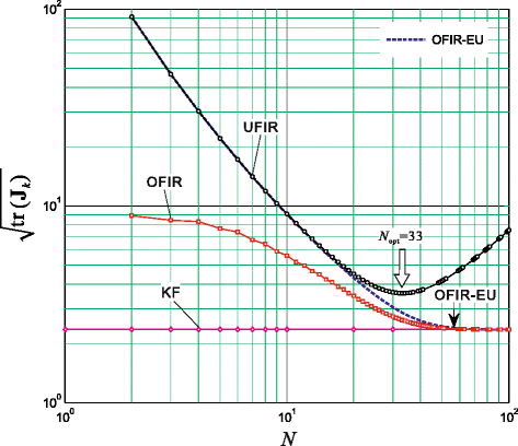
Typical RMSEs as functions of N for different filters with \({\sigma _{w}^{2}}=1\)
Fig. 2 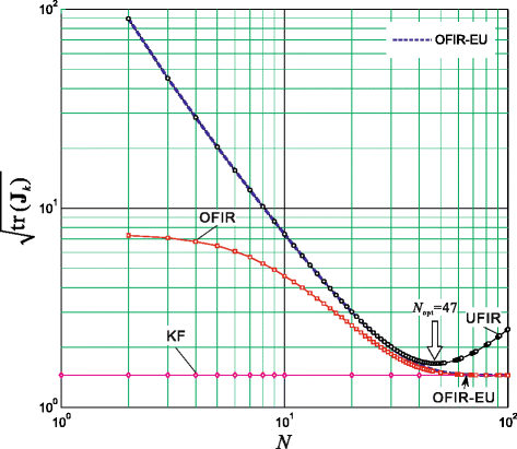
Typical RMSEs as functions of N for different filters with \({\sigma _{w}^{2}}=0.1\)
-
–
The OFIR and OFIR-EU estimates converge to the KF estimate by increasing the averaging horizon N. The estimates become practically indistinguishable when N≫N opt.
-
–
An increase in N opt diminishes the error difference between the OFIR and UFIR filters (compare Fig. 1 with N opt=33 and Fig. 2 with N opt=47).
-
–
Because the MSEs in the OFIR and OFIR-EU filters diminish with N, these filters are full-horizon [18].


Filtering with errors in the noise statistics
The noise statistics required by the KF are commonly not completely know to the engineer. In order to investigate the effect of the imprecisely defined noise covariances in the worst case, we introduce a correction coefficient p as p 2 Q and R/p 2, vary p from 0.1 to 10, and plot the RMSE \(\sqrt {\text {tr}\,\mathbf {J}_{k}}\) as shown in Fig. 3.

Typical RMSE \(\sqrt {\text {tr}\,\mathbf {J}_{k}}\) as a function of p for KF and FIR filters
Note that the MSE functions of optimal filters are inherently concave on p with a minimum at p=1 and the MSE of the UFIR filter is p-invariant.
As expected, p=1 makes the OFIR filter, OFIR-EU filter, and KF a bit more accurate than the UFIR filter. But, that is only within a narrow range of p (0.6<p<1.5 in Fig. 3) that the KF slightly outperforms the UFIR filter. Otherwise, the UFIR filter demonstrates smaller errors. Referring to practical difficulties in the determination of noise statistics [7], the latter can be considered as an important engineering advantage of the UFIR filter. Some other generalizations also emerge from Fig. 3:
-
–
The embedded unbiasedness makes the OFIR-EU filter p-invariant with p<1. In this sense, the OFIR-EU is equal here to the UFIR filter, and this can be considered as a particular meaningful property of the approach proposed.
-
–
With p<1, the KF is more sensitive to errors in the noise statistics than the FIR filters.
-
–
By p>1, the MSEs in the KF, OFIR filter, and OFIR-EU filter grow and converge.
Overall, we conclude that the OFIR-EU filter inherits the robustness of the UFIR filte against the noise statistics and has better performance than the OFIR filter and KF.
Filtering with model uncertainties
To learn effect of the temporary model uncertainties on the filtering accuracy, in this section we set τ=0.1 s when 160≤k≤180 and τ=0.05 s otherwise. The noise variances are allowed to be \(\sigma _{w1}^{2} = 1\), \(\sigma _{w2}^{2} = 1/ \mathrm {s}^{2}\), and \({\sigma _{v}^{2}} = 10\). The process is simulated at 400 subsequent points.
Typical filtering estimates are sketched in Fig. 4. As can be seen, the OFIR-EU filter (case p=0.2) and the UFIR filter produce almost equal errors and demonstrate good robustness against the uncertainties. Just on the contrary, the KF demonstrates much worse robustness for any p≤1.

Instantaneous estimation errors caused by the temporary model uncertainties with p<1 for the KF, UFIR filter, and OFIR-EU filter
7 Conclusions
Summarizing, we notice that the unbiasedness imbedded to the OFIR filter instills into it several useful properties. Unlike the OFIR filter, the OFIR-EU filter completely ignores the initial conditions. The OFIR-EU filter is equivalent to the MVU FIR filter. In terms of accuracy, the OFIR-EU filter is in between the UFIR and OFIR filters. Unlike in the UFIR filter which MSE is minimized by N opt, MSEs in the OFIR-EU and OFIR filters diminish with N and these filters are thus full-horizon. The performance of OFIR-EU filter is developed by varying the horizon N around N opt or ranging the correction coefficient p around p=1. Accordingly, the OFIR-EU filter in general demonstrates higher immunity against errors in the noise statistics and better robustness against temporary model uncertainties than the OFIR filter and KF.
Referring to the fact that optimal FIR filters are essentially the full-horizon filters but their batch forms are computationally inefficient, we now focus our attention on the fast iterative form for OFIR-EU filter and plan to report the results in near future.
8 Endnote
1 \(\hat {\mathbf {x}}_{k|k}\) means the estimate at k via measurements from the past to k.
9 Appendix A: Proof of Lemma 1
Represent the performance criterion in (21) as
By partitioning K as K T= [ k 1 k 2⋯k m ], where m is the dimension of K, rewrite ϕ as
in which
where g i and m i are the ith column vector of G and M, respectively, and i=1,2,…,m. Reasoning along similar lines, the ith constraint can be specified by
Now note that ϕ i and \({\mathfrak {L}^{i}_{\left \{ {\mathbf {U}^{T}\mathbf {k}_{i}} = \mathbf {z}_{i}\right \} \left | \theta \right.}}\) are independent on k j , j≠i, and the optimization problem (21) can be reduced to m independent optimization problems as
where i=1,2,…,m. Now, define an auxiliary function φ i|θ as
where λ i denotes the ith vector of the Lagrange multiplier. Note that φ i|θ depends on θ which governs the existing of constraint. Setting θ=1, first consider a general case of F≠U, L≠U, G≠Z and M≠Z which is denoted as case (a). Taking the derivative of φ i|a with respect to k i and λ i respectively and making them equal to zero lead to
which can further be rewritten as
where \(\mathbf {\Xi }_{a} \buildrel \Delta \over = \mathbf {FHF}^{T}+\mathbf {LPL}^{T}+\mathbf {S}\), H>0, P>0, and S>0. By multiplying the both sides of (89) with U T from the left-hand side, using the constraint (85), and arranging the terms, arrive at
Substituting (90) into (89) and taking into account that H=H T, P=P T, S=S T and \(\mathbf {\Xi }_{a}=\mathbf {\Xi }_{a}^{T}\), transforms \(\mathbf {k}_{i}^{T}\) to
At this point, reconstruct K a as
In the case of θ=1, F=U and H=Z which is denoted as case (b) or θ=1, G=U and M=Z which is denoted as case (c), the solutions can be obtained similarly to case (a), respectively,
with
Note that (93) and (94) are equal to the results found in [11] for the receding horizon FIR filtering via prediction state model.
In the case of θ=0 which is denoted as case (d), the derivative of φ i|d with respect to k i|d becomes
where Ξ d =Ξ a , and yields
Then K d can be found to be
Finally, by observing that
when F=U and L=U, and using θ as an indicating parameter of the constraint, matrices K a , K b , K c , and K d can be unified with
where Ξ is specified by (23). An equivalent form of (100) is (22) and the proof is complete.
References
CF Gauss, Theory of the combination of observations least subject to errors. (SIAM Publ, Philadelphia, 1995). Transl. by Stewart GW.
H Stark, JW Woods, Probability, random processes, and estimation theory for engineers, 2nd edn (Prentice Hall, Upper Saddle River, NJ, 1994).
JH Stapleton, Linear statistical models, 2nd edn (Wiley, New York, 2009).
AC Aitken, On least squares and linear combinations of observations. Proc. R. Soc. Edinb. 55, 42–48 (1935).
SM Kay, Fundamentals of statistical signal processing (Prentice Hall, New York, 2001).
YS Shmaliy, An unbiased FIR filter for TIE model of a local clock in applications to GPS-based timekeeping. IEEE Trans. Ultrason. Ferroelec. Freq. Control. 53(5), 862–870 (2006).
BP Gibbs, Advanced Kalman filtering, least-squares and modeling (John Wiley & Sons, Hoboken, NJ, 2011).
M Hardy, An illuminating counterexample. Am. Math. Mon. 110(3), 232–238 (2003).
D Simon, Optimal state estimation: Kalman, Hinf, and nonlinear approaches (John Wiley & Sons, Honboken, NJ, 2006).
AH Jazwinski, Stochastic processes and filtering theory (Academic, New York, 1970).
WH Kwon, S Han, Receding horizon control: model predictive control for state models (Springer, London, 2005).
YS Shmaliy, Linear optimal FIR estimation of discrete time-invariant state-space models. IEEE Trans. Signal Process. 58(6), 3086–2010 (2010).
KR Johnson, Optimum, linear, discrete filtering of signals containing a nonrandom component. IRE Trans. Inf. Theory. 2(2), 49–55 (1956).
AH Jazwinski, Limited memory optimal filtering. IEEE Trans. Autom. Contr. 13(10), 558–563 (1968).
CK Ahn, S Han, WH Kwon, FIR filters for linear continuous-time state-space systems. IEEE Signal Process. Lett. 13(9), 557–560 (2006).
WH Kwon, PS Kim, P Park, A receding horizon Kalman FIR filter for discrete time-invariant systems. IEEE Trans. Autom. Contr. 99(9), 1787–1791 (1999).
WH Kwon, PS Kim, S Han, A receding horizon unbiased FIR filter for discrete-time state space models. Automatica. 38(3), 545–551 (2002).
YS Shmaliy, An iterative Kalman-like algorithm ignoring noise and initial conditions. IEEE Trans. Signal Process. 59(6), 2465–2473 (2011).
YS Shmaliy, Optimal gains of FIR estimations for a class of discrete-time state-space models. IEEE Signal Process. Lett. 15, 517–520 (2008).
CK Ahn, Strictly passive FIR filtering for state-space models with external disturbance. Int. J. Electron. Commun. 66(11), 944–948 (2012).
JM Park, CK Ahn, MT Lim, MK Song, Horizon group shift FIR filter: alternative nonlinear filter using finite recent measurement. Measurement. 57, 33–45 (2014).
CK Ahn, PS Kim, Fixed-lag maximum likelihood FIR smoother for state-space modelsIEICE Electron. IEICE Electron. Express. 5(1), 11–16 (2008).
YS Shmaliy, LJ Morales-Mendoza, FIR Smoothing of discrete-time polynomial signals in state space. IEEE Trans. Signal Process. 58(5), 2544–2555 (2010).
BK Kwon, S Han, OK Kim, WH Kwon, Minimum variance FIR smoothers for discrete-time state space models. EEE Trans. Signal Process. Lett. 14(8), 557–560 (2007).
L Danyang, L Xuanhuang, Optimal state estimation without the requirement of a prior statistics informantion of the initial state. IEEE Trans. Autom. Contr. 39(10), 2087–2091 (1994).
KV Ling, KW Lim, Receding horizon recursive state estimation. IEEE Trans. Autom. Contr. 44(9), 1750–1753 (1999).
J Makhoul, Linear prediction: a tutorial review. Proc. IEEE. 63, 561–580 (1975).
J Levine, The statistical modeling of atomic clocks and the design of time scales. Rev. Sci. Instrum. 83, 021101–1–021101-28 (2012).
Y Kou, Y Jiao, D Xu, M Zhang, Ya Liu, X Li, Low-cost precise measurement of oscillator frequency instability based on GNSS carrier observation. Adv. Space Res. 51(6), 969–977 (2013).
JW Choi, S Han, JM Cioffi, An FIR channel estimation filter with robustness to channel mismatch condition. IEEE Trans. Broadcast. 54(1), 127–130 (2008).
J Salmi, A Richter, V Koivunen, Detection and tracking of MIMO propagation path parameters using state-space approach. IEEE Trans. Signal Process. 57(4), 1538–1550 (2009).
I Nevat, J Yuan, Joint channel tracking and decoding for BICM-OFDM systems using consistency test and adaptive detection selection. IEEE Trans. Veh. Technol. 58(8), 4316–4328 (2009).
YS Shmaliy, Unbiased FIR filtering of discrete-time polynomial state-space models. IEEE Trans. Signal Process. 57(4), 1241–1249 (2009).
YS Shmaliy, O Ibarra-Manzano, Time-variant linear optimal finite impulse response estimator for discrete state-space models. Int. J. Adapt. Contrl Signal Process. 26(2), 95–104 (2012).
YS Shmaliy, Suboptimal FIR filtering of nonlinear models in additive white Gaussian noise. IEEE Trans. Signal Process. 60(10), 5519–5527 (2012).
D Simon, YS Shmaliy, Unified forms for Kalman and finite impulse response filtering and smoothing. Automatica. 49(6), 1892–1899 (2013).
YL Wei, J Qiu, HR Karimi, M Wang, A new design of H ∞ filtering for continuous-time Markovian jump systems with time-varying delay and partially accessible mode information. Signal Process. 93(9), 2392–2407 (2013).
YL Wei, M Wang, J Qiu, New approach to delay-dependent H α filtering for discrete-time Markovian jump systems with time-varying delay and incomplete transtion descriptions. IET Control Theory Appl. 7(5), 684–696 (2013).
J Qiu, YL Wei, HR Karimi, New approach to delay-dependent H α control for continuous-time Markovian jump systems with time-varying delay and deficient transtion descriptions. J. Frankl. Inst. 352(1), 189–215 (2015).
S Zhao, YS Shmaliy, B Huang, F Liu, Minimum variance unbiased FIR filter for discrete time-variant models. Automatica. 53, 355–361 (2015).
PS Kim, An alternative FIR filter for state estimation in discrete-time systems. Digit. Signal Process. 20(3), 935–943 (2010).
FR Echeverria, A Sarr, YS Shmaliy, Optimal memory for discrete-time FIR filters in state-space. IEEE Trans. Signal Process. 62, 557–561 (2014).
Acknowledgements
This investigation was supported by the Royal Academy of Engineering under the Newton Research Collaboration Programme NRCP/1415/140.
Author information
Authors and Affiliations
Corresponding author
Additional information
Competing interests
The authors declare that they have no competing interests.
Rights and permissions
Open Access This article is distributed under the terms of the Creative Commons Attribution 4.0 International License (http://creativecommons.org/licenses/by/4.0/), which permits unrestricted use, distribution, and reproduction in any medium, provided you give appropriate credit to the original author(s) and the source, provide a link to the Creative Commons license, and indicate if changes were made.
About this article

Cite this article
Zhao, S., Shmaliy, Y.S., Liu, F. et al. Effect of embedded unbiasedness on discrete-time optimal FIR filtering estimates. EURASIP J. Adv. Signal Process. 2015, 83 (2015). https://doi.org/10.1186/s13634-015-0268-0
Received:
Accepted:
Published:
DOI: https://doi.org/10.1186/s13634-015-0268-0