A Bayesian network approach to linear and nonlinear acoustic echo cancellation

Abstract

This article provides a general Bayesian approach to the tasks of linear and nonlinear acoustic echo cancellation (AEC). We introduce a state-space model with latent state vector modeling all relevant information of the unknown system. Based on three cases for defining the state vector (to model a linear or nonlinear echo path) and its mathematical relation to the observation, it is shown that the normalized least mean square algorithm (with fixed and adaptive stepsize), the Hammerstein group model, and a numerical sampling scheme for nonlinear AEC can be derived by applying fundamental techniques for probabilistic graphical models. As a consequence, the major contribution of this Bayesian approach is a unifying graphical-model perspective which may serve as a powerful framework for future work in linear and nonlinear AEC.

1 Introduction

The problem of acoustic echo cancellation (AEC) is one of the earliest applications of adaptive filtering to acoustic signals and yet is still an active research topic [1, 2]. Especially in applications like teleconferencing and hands-free communication systems, it is of vital importance to compensate acoustic echos and thus prevent the users from listening to delayed version of their own speech [3]. Since the invention of the normalized least mean square (NLMS) algorithm in 1960 [4], the acoustic coupling between loudspeakers and microphones is often modeled by adaptive linear finite impulse response (FIR) filters. However, the statistical properties of speech signals (being wide-sense stationary only for short time frames) and challenging properties of the acoustic environment (such as speech signals as interference, non-stationary background noise and time-varying acoustic echo paths) complicate the filter adaptation and motivated various concepts improving the performance of linear FIR filters in many practical scenarios [5–7]. Despite these challenges, single-channel linear AEC has already reached a mature state as vital part of modern communication devices. On the other hand, the nonlinear distortions created by amplifiers and transducers in miniaturized loudspeakers require dedicated nonlinear echo-path models and are still a very active research topic [8, 9]. In this context, a variety of concepts for nonlinear AEC have been proposed based on artificial neural networks [10, 11], Volterra filters [12, 13], or Kernel methods [14, 15]. A commonly used model, which is also considered in this article, is a cascade of a nonlinear memoryless preprocessor (to model the loudspeaker signal distortions) and an adaptive linear FIR filter (to model the acoustic sound propagation and the microphone) [9, 16–19].

Recently, the application of machine learning techniques to signal processing tasks attracted increasing interest [20–22]. In particular, graphical models provide a powerful framework for deriving (links between) numerous existing algorithms based on probabilistic inference [23–25]. Besides the widely used factor graphs, which capture detailed information about the factorization of a joint probability distribution [23, 26, 27], especially directed graphical models, such as Bayesian networks, have been shown to be well-suited for modeling causal probabilistic relationships of sequential data like speech [28, 29].

This article provides a concise overview on different algorithms for linear and nonlinear AEC from a unifying Bayesian network perspective. For this, we consider a state-space model with a latent (unobserved) state vector capturing all relevant information of the unknown system. Depending on the definition of the state vector (modeling a linear or nonlinear echo path) and its mathematical relation to the observation, we illustrate that the application of different probabilistic inference techniques to the same graphical model straightforwardly leads to the NLMS algorithm with fixed/adaptive stepsize value, the Hammerstein group model (considered from this perspective here for the first time), and a numerical sampling scheme for nonlinear AEC. This consistent Bayesian view on conceptually different algorithms highlights the probabilistic assumptions underlying the respective derivations and provides a powerful framework for further research in linear and nonlinear AEC.

Throughout this article, the problem of AEC is considered in the time domain (time index n), where we denote scalars z _n by lowercase italic letters, column vectors z _n by lower case bold letters, and matrices C _z,n by upper case bold letters. Furthermore, sequences of variables are written as z _1:N ={z ₁,…,z _N }. For a normally distributed random vector z _n with mean vector μ _z,n and covariance matrix C _z,n , we write

$$\mathbf{z}_{n}\sim \mathcal{N} \left\{\mathbf{z}_{n} | \boldsymbol{\mu}_{\mathbf{z},n},\mathbf{C}_{\mathbf{z},n}\right\}. $$

Note that C _z,n =C _z,n I (identity matrix I) implies the elements of z _n to be mutually statistically independent and of equal variance C _z,n . Finally, we distinguish between the probability density function (PDF) p(z _n ) and realizations $z_{n}^{(l)}$ (samples drawn from p(z _n )) of a random variable z _n , where l is the sample index.

This article is structured as follows: First, we briefly review Bayesian networks and introduce a general state-space model in Section 2. This state-space model will be further specified in Section 3 for the tasks of linear and nonlinear AEC. This is followed by applying several fundamental probabilistic inference techniques for deriving the NLMS algorithm with fixed/adaptive stepsize value (linear AEC, Section 4), as well as the Hammerstein group model and a numerical sampling scheme (nonlinear AEC, Section 5). Finally, the practical performance of the algorithms is illustrated in Section 6 and conclusions are drawn in Section 7.

2 Review of Bayesian networks and state-space modeling

This section provides a concise review of Bayesian networks and state-space modeling following the detailed discussions in [30].

2.1 Bayesian networks

Bayesian networks are graphical descriptions of joint probability distributions and provide a powerful framework for many kinds of regression and classification problems. Consisting of nodes (random variables) and directed links (probabilistic relationships), they define the factorization properties of a joint PDF p(z _1:K ) through the following rule:

$$\begin{array}{@{}rcl@{}} p(z_{1:K}) = \prod\limits_{k=1}^{K} p\left(z_{k} | \,\text{par}(z_{k})\right), \end{array} $$

((1))

where {par(z _k )} is the set of nodes (so-called parent nodes of z _k ) from which a link is going to the node z _k . We illustrate this basic definition by the example shown in Fig. 1: the joint PDF p(z ₁,z ₂,z ₃) over the random variables z ₁, z ₂, z ₃ factorizes to

$$\begin{array}{@{}rcl@{}} p(z_{1}, z_{2}, z_{3}) = p(z_{1}) \; p(z_{2}|z_{1}) \; p(z_{3}|z_{1}, z_{2}), \end{array} $$

((2))

Fig. 1

Example of a Bayesian network

where the PDF of each random variable is conditioned on its parent nodes (if any). This fundamental factorization property of Bayesian networks can be employed to derive several rules of conditional dependence and independence for Bayesian networks. As an example, we consider three independent random variables z ₁, η, ε defining two further random variables z ₂ and z ₃ through the following observation model:

$$ z_{2} = z_{1} + \varepsilon, \quad z_{3} = z_{2} + \eta. $$

((3))

The probabilistic relationship of z ₁,z ₂,z ₃ can be represented by the Bayesian network depicted in Fig. 2 a, where the variables η and ε have been omitted to focus on the head-to-tail relationship in z ₂. Although z ₁ and z ₃ are statistically dependent, we can exploit (1) to show that z ₁ and z ₃ are conditionally independent given z ₂:

$$\begin{array}{*{20}l} p(z_{1}, z_{3} | z_{2}) &= \frac{p(z_{1}, z_{2}, z_{3})}{p(z_{2})} \end{array} $$

((4))

Fig. 2

Bayesian networks with a) head-to-tail, b) tail-to-tail, and c) head-to-head relationship in z ₂ [31]

$$\begin{array}{*{20}l} & \stackrel{(1)}{=} \frac{p(z_{1}) \; p(z_{2} | z_{1}) \; p(z_{3}|z_{2})}{p(z_{2})} \\ &= p(z_{1}|z_{2}) \; p(z_{3}|z_{2}). \end{array} $$

((5))

The same property of conditional independence can be derived for the case of a tail-to-tail relationship in z ₂ as shown in Fig. 2 b. In contrast, two independent random variables z ₁ and z ₃ are conditionally dependent given z ₂ if they share a head-to-head relationship as in Fig. 2 c, which would, e.g., be the case if z ₂ was defined as z ₂=z ₁+z ₃.

Generalizing the above, it can be shown that two random variables z ₁ and z ₃ are conditionally independent given a set of random variables C if all paths leading from z ₁ to z ₃ contain a node, where the

• arrows meet head-to-tail or tail-to-tail, and the node is in the set C

• arrows meet head-to-head and neither the node, nor any of its descendants, are in the set C [30].

2.2 State-space modeling

In this part, we introduce a general probabilistic model (later applied to linear and nonlinear AEC) and review fundamental techniques which are commonly employed in Bayesian network modeling.

Probabilistic model: Assume all relevant information of an unknown system at time instant n is captured by a latent (unobserved) state vector

$$ \mathbf{z}_{n}= \,[\!z_{0,n},z_{1,n},\ldots,z_{R-1,n}]^{\mathrm{T}}. $$

((6))

In general, a state-space model is defined by the process equation (modeling the temporal evolution of the state vector) and the observation equation (modeling the relation between state vector and observation). The remainder of this article is based on the following observation equation and state equation, respectively,

$$ d_{n} = \mathbf{g} \left(\mathbf{x}_{n},\mathbf{z}_{n} \right) +v_{n} \quad \text{and} \quad \mathbf{z}_{n} = \mathbf{z}_{n-1} + \mathbf{w}_{n}, $$

((7))

where the temporal evolution of the state vector z _n is captured by the additive uncertainty w _n . Furthermore, the observation d _n in (7) is modeled by adding a scalar uncertainty v _n to the output of the function g(x _n ,z _n ), which depends on the state vector z _n and the input signal vector x _n = [ x _n ,x _n−1,…,x _n−M+1]^T (time-domain samples x _n at time instant n). The state-space model of (7) is represented by the Bayesian network in Fig. 3, where observed variables, such as d _n , are marked by shaded circles. Note that the input signal vector x _n is regarded as an observed random variable (without explicitly estimated statistics) and thus omitted in Fig. 3 for notational convenience in the later probabilistic calculus. The conditional independence rules of Section 2 reveal two major properties of the Bayesian network in Fig. 3:

• With respect to the latent state vector z _n−1, the head-to-tail relationships of all paths from d _1:n−2 to z _n and the tail-to-tail relationship of the path from d _n−1 to z _n together imply the current state vector z _n to depend on all previous observations d _1:n−1. For the conditional PDF of z _n given {z _n−1,d _1:n−1}, this leads to:

  $$ p \left(\mathbf{z}_{n} | \mathbf{z}_{n-1}, d_{1:n-1}\right) = p \left(\mathbf{z}_{n} |\mathbf{z}_{n-1}\right). $$

  ((8))

  Fig. 3

  

  Bayesian network of the state-space model in (7), where the observations d _1:n are marked by coloration [30]

• The current observation d _n depends on all previous observations d _1:n−1 following the head-to-tail relationship in the latent state vector z _n . This allows to reformulate the conditional PDF of d _n given {z _n ,d _1:n−1} as

  $$ p \left(d_{n} | \mathbf{z}_{n}, d_{1:n-1}\right) = p \left(d_{n} |\mathbf{z}_{n}\right). $$

  ((9))

The state-space model in (7) is a fundamental probabilistic model and will be employed to derive well-known methods for linear and nonlinear AEC in Sections 4 and 5. For this, we make the following assumptions on the PDFs of the additive uncertainties in (7) [32]:

• w _n is normally distributed with mean vector 0 and covariance matrix C _w,n defined by the scalar variance C _w,n :

  $$ \mathbf{w}_{n} \sim \mathcal{N} \{\mathbf{w}_{n} | \mathbf{0}, \mathbf{C}_{\mathbf{w}, n}\},\quad \mathbf{C}_{\mathbf{w},n} = C_{\mathbf{w},n} \mathbf{I}. $$

  ((10))

• v _n is assumed to be normally distributed with variance C _v,n and zero mean:

  $$ v_{n} \sim \mathcal{N} \{ v_{n} | 0, C_{v, n}\}. $$

  ((11))

To derive estimates for the state vector and the hyperparameters C _v,n and C _w,n , we recall the steps of probabilistic inference and learning in the next part.

Inference/Learning: In the inference stage, the mean vector of the posterior PDF $p \left (\mathbf {z}_{n} | d_{1:n}\right)$ can be identified as minimum mean square error (MMSE) estimate for the state vector [30]:

$$ \hat{\mathbf{z}}_{n} = \underset{\tilde{\mathbf{z}}_{n}}{\operatorname{argmin}} \; \mathcal{E} \left\{ ||\tilde{\mathbf{z}}_{n}-\mathbf{z}_{n} ||_{2}^{2} \right\} = \mathcal{E} \left\{ \mathbf{z}_{n} | d_{1:n} \right\}, $$

((12))

where ||·||₂ is the Euclidean norm and $\mathcal {E}\{\cdot \}$ the expectation operator. Note that this MMSE estimate can be calculated in an analytically closed form in case of linear relations between the variables in (7) and is optimal in the Bayesian sense for jointly normally distributed random variables z _n and d _1:n .

In the learning stage, the hyperparameters C _v,n and C _w,n of the state-space model in (7) are estimated by solving a maximum likelihood (ML) problem (see Section 4.1 for more details).

3 State-space model for linear and nonlinear AEC

To identify the electroacoustic echo path (from the loudspeaker to the microphone), a physically justifiable model has to be selected first. As the sound propagation through air can be modeled by a linear system [1], the acoustic path at time n between loudspeaker and microphone is estimated by the linear FIR filter

$$ \hat{\mathbf{h}}_{n}=\left[\hat{h}_{0,n},\hat{h}_{1,n},\ldots,\hat{h}_{M-1,n}\right]^{\mathrm{T}} $$

((13))

of length M. Ideally, the error signal

$$ e_{n}=d_{n}-\hat{d}_{n} $$

((14))

between the observation d _n and the linear transformation of the input vector y _n :

$$ \hat{d}_{n} = \hat{\mathbf{h}}_{n-1}^{\mathrm{T}} \mathbf{y}_{n} $$

((15))

equals zero, which means that the estimated impulse response matches the actual physical one. In many practical applications, nonlinear loudspeaker signal distortions created by amplifiers and transducers in minituarized loudspeakers prior to the linear acoustic impulse response limit the practical performance of linear echo path models. This justifies to model the overall echo path by a nonlinear-linear cascade of a memoryless preprocessor (to model nonlinear loudspeaker signal distortions) preceding the linear FIR filter $\hat {\mathbf {h}}_{n}$ (to model the sound propagation through air) [9, 16, 17], see Fig. 4. Motivated by the good performance in nonlinear AEC [18, 19, 32], we choose a polynomial preprocessor

Fig. 4

Nonlinear AEC scenario with memoryless preprocessor $\mathbf {f}(\mathbf {x}_{n},\hat {\mathbf {a}}_{n-1})$ and linear FIR filter $\hat {\mathbf {h}}_{n-1}$

$$ \mathbf{y}_{n} = \mathbf{f}(\mathbf{x}_{n},\hat{\mathbf{a}}_{n-1}) = \mathbf{x}_{n} + \sum_{\nu=1}^{P} \hat{a}_{\nu,n-1} \Phi_{\nu} \{\mathbf{x}_{n}\}, $$

((16))

defined as weighted superposition of nonlinear functions Φ _ν {·} parameterized by the estimated vector

$$ \hat{\mathbf{a}}_{n-1}=\left[\hat{a}_{1,n-1},\hat{a}_{2,n-1},\ldots,\hat{a}_{P,n-1}\right]^{\mathrm{T}}, $$

((17))

to perform an element-wise transformation of the loudspeaker signal vector x _n to the input vector y _n of the linear FIR filter in (15). In particular, odd-order Legendre functions of the first kind (inserted for Φ _ν {·} in (16)) have been shown to be efficient for specific applications [18, 19]. By combining (15) and (16), the error signal e _n resulting from the nonlinear-linear cascade in Fig. 4 is given as:

$$ \hat{d}_{n} = \hat{\mathbf{h}}_{n-1}^{\mathrm{T}} \left(\mathbf{x}_{n} + \sum_{\nu=1}^{P} \hat{a}_{\nu,n-1} \Phi_{\nu} \{\mathbf{x}_{n}\} \right). $$

((18))

It is obvious that the nonlinear-linear cascade in Fig. 4 simplifies to a linear AEC system when setting the estimated preprocessor coefficients equal to zero because:

$$ \mathbf{y}_{n} \stackrel{(16)}{=} \mathbf{x}_{n}, \quad \text{for} \quad \; \hat{\mathbf{a}}_{n-1}=\,[\!0,0,\ldots,0]^{\mathrm{T}}. $$

((19))

In the following, we describe the tasks of linear and nonlinear AEC from a Bayesian network perspective by further specializing the general state-space model in (7). This is summarized in Fig. 5 as guidance through the following derivations.

Fig. 5

Overview of the following sections including the different observation equations and respective state-vector definitions for the tasks of linear and nonlinear AEC, where the process equation equals z _n =z _n−1+w _n for all cases

Linear AEC: The observation equation for linear AEC follows the definition of $\hat {d}_{n}$ in (15):

$$ d_{n} = \mathbf{z}_{n}^{\mathrm{T}} \mathbf{x}_{n} + v_{n}, \quad \text{with} \quad \mathbf{z}_{n} = \mathbf{h}_{n}, $$

((20))

where the latent length-M vector h _n models the acoustic path between the loudspeaker and the microphone. Note that the observation equation in (20) is denoted as a model which is linear in the coefficients (LIC model) due to the linear relation between the elements of the state vector z _n and the observation d _n .

Nonlinear AEC: For the task of nonlinear AEC, we derive the observation equation from (18):

$$ d_{n} = \mathbf{h}_{n}^{\mathrm{T}} \left(\mathbf{x}_{n} + \sum_{\nu=1}^{P} a_{\nu,n} \Phi_{\nu} \{\mathbf{x}_{n}\} \right) + v_{n}, $$

((21))

where the latent variables a _ν,n (ν=1,…,P) model the preprocessor coefficients and represent the entries of the length-P vector a _n , which is identically defined as in (17). Depending on the choice of the state vector, the observation equation in (21) represents a LIC model or a model which is nonlinear in the coefficients (NIC model) of the state vector. To start with the latter case, we specify:

$$ \mathbf{z}_{n}=\left[\mathbf{a}^{\mathrm{T}}_{n}, \mathbf{h}^{\mathrm{T}}_{n}\right]^{\mathrm{T}} $$

((22))

as state vector of length M+P. Thereby, the observation equation in (21) becomes a NIC model due to the nonlinear relation between the entries of the state vector z _n and the observation d _n . Alternatively, we can express the same input-output relation by the length- M·(P+1) state vector

$$\begin{array}{*{20}l} \mathbf{z}_{n}&=\left[\mathbf{h}^{\mathrm{T}}_{n},a_{1,n} \mathbf{h}^{\mathrm{T}}_{n},\ldots,a_{P,n} \mathbf{h}^{\mathrm{T}}_{n}\right]^{\mathrm{T}} \end{array} $$

((23))

together with the observation equation

$$ d_{n} = \mathbf{z}_{n}^{\mathrm{T}} \left[ \mathbf{x}_{n}^{\mathrm{T}}, \Phi_{1} \{\mathbf{x}_{n}\}^{\mathrm{T}},\ldots, \Phi_{P} \{\mathbf{x}_{n}\}^{\mathrm{T}}\right]^{\mathrm{T}} + v_{n}. $$

((24))

This represents a LIC model as the output d _n linearly depends on the coefficients of z _n . The three previously described pairs of observation equations and state vector definitions represent special cases of the state-space model in (7) and will be employed in the subsequent sections to derive algorithms for linear and nonlinear AEC following the schematic overview in Fig. 5.

4 A Bayesian view on linear AEC

Consider the task of linear AEC using the state-space model (see left part of Fig. 5)

$$ d_{n} = \mathbf{h}_{n}^{\mathrm{T}} \mathbf{x}_{n} + v_{n}, \quad \mathbf{h}_{n} = \mathbf{h}_{n-1} + \mathbf{w}_{n}, $$

((25))

which can be represented by the Bayesian network shown in Fig. 6. To derive an NLMS-like filter adaptation, we assume the PDFs $p\left (\mathbf {h}_{n} | \mathbf {h}_{n-1}\right)$, $p\left (d_{n} | \mathbf {h}_{n}\right)$, and $p \left (\mathbf {h}_{n} | d_{1:n}\right)$ to be Gaussian probability distributions [30], where the latter is denoted as:

$$ p \left(\mathbf{h}_{n} | d_{1:n}\right) \stackrel{(12)}{=} \mathcal{N} \left\{ \mathbf{h}_{n} | \hat{\mathbf{h}}_{n},\mathbf{C}_{\mathbf{h},n} \right\}. $$

((26))

Fig. 6

Bayesian network of the state-space model in (25), where the observations d _1:n are marked by coloration [30]

Therein, we restrict the covariance matrix of $p \left (\mathbf {h}_{n} | d_{1:n}\right)$ to be diagonal [33]

$$ \mathbf{C}_{\mathbf{h},n} = C_{\mathbf{h},n} \mathbf{I} \quad \text{with} \quad C_{\mathbf{h},n} = \text{tr}\{\mathbf{C}_{\mathbf{h},n}\}/M, $$

((27))

where tr{·} represents the trace of a matrix. This implies the filter taps to be uncorrelated and of equal estimation uncertainty. The assumption (27) will be the basis for deriving the NLMS algorithm with adaptive (Section 4.1) and fixed (Section 4.2) stepsize value.

4.1 NLMS algorithm with adaptive stepsize value [32]

The NLMS algorithm with optimal stepsize calculation has been initially proposed by Yamamoto and Kitayama in 1982 [34]. Since then, the derivation of the adaptive stepsize NLMS algorithm with filter update

$$ \hat{\mathbf{h}}_{n} = \hat{\mathbf{h}}_{n-1} + \frac{1}{M} \frac{\mathcal{E}\left\{ ||\mathbf{h}_{n} - \hat{\mathbf{h}}_{n-1} ||^{2}_{2} \right\}}{\mathcal{E}\left\{{e_{n}^{2}}\right\}} \mathbf{x}_{n} e_{n} $$

((28))

has been adopted in many textbooks [35]. As the true echo path h _n is not observable, the numerator in (28) can be approximated by introducing a delay of N _T coefficients to the echo path h _n [36, 37]. Then, it is assumed that the leading N _T coefficients $\hat {h}_{\kappa,n-1}$, with κ=0,…,N _T −1, should be zero for causal systems and any nonzero coefficient values are representative for the system error norm $\mathcal {E}\left \{ ||\mathbf {h}_{n} - \hat {\mathbf {h}}_{n-1} ||^{2}_{2} \right \}$. Typically, the denominator in (28) is recursively approximated using a smoothing factor η [35, 37]. Thus, the filter update is realized as follows:

$$\begin{array}{*{20}l} \hat{\mathbf{h}}_{n} &= \hat{\mathbf{h}}_{n-1} + \frac{1}{ N_{T}} \frac{ \sum\limits_{\kappa=0}^{N_{T}-1} \hat{h}^{2}_{\kappa,n-1} }{ (1-\eta) {e_{n}^{2}} + \eta \mathcal{E}\left\{e_{n-1}^{2}\right\}} \mathbf{x}_{n} e_{n} \notag \\ &= \hat{\mathbf{h}}_{n-1} + \beta_{n} \mathbf{x}_{n} e_{n}. \end{array} $$

((29))

However, the approximations in (29) often lead to oscillations which have to be addressed by limiting the absolute value of β _n [36].

In the following, we employ Bayesian network modeling to derive the filter update of (28) (in the inference stage) and an estimation scheme for the adaptive stepsize β _n (in the learning stage).

Inference: To derive the MMSE estimate of the state vector following (12), we rewrite the posterior PDF as

$$\begin{array}{*{20}l} p(\mathbf{h}_{n}|d_{1:n}) &= \frac{p(d_{n}, \mathbf{h}_{n} | d_{1:n-1}) }{ p(d_{n} | d_{1:n-1})} \end{array} $$

((30))

$$\begin{array}{*{20}l} &= \frac{p(d_{n} | \mathbf{h}_{n},d_{1:n-1}) p(\mathbf{h}_{n} | d_{1:n-1}) }{ p(d_{n} | d_{1:n-1})} \end{array} $$

((31))

$$\begin{array}{*{20}l} &\stackrel{(8)}{=} \frac{p(d_{n} | \mathbf{h}_{n}) p(\mathbf{h}_{n} | d_{1:n-1}) }{ p(d_{n} | d_{1:n-1})}. \end{array} $$

((32))

Then, the product rules of linear Gaussian models ([30] p. 639) can be applied to derive recursive updates for the mean vector $\hat {\mathbf {h}}_{n} = \mathcal {E}(\mathbf {h}_{n}|d_{1:n})$ and the covariance matrix C _h,n , resulting in a special case of the well-known Kalman filter equations:

$$\begin{array}{*{20}l} &\hat{\mathbf{h}}_{n} = \hat{\mathbf{h}}_{n-1} + \frac{(\mathbf{C}_{\mathbf{h},n-1} +\mathbf{C}_{\mathbf{w},n}) \mathbf{x}_{n} e_{n}}{\mathbf{x}^{\mathrm{T}}_{n} (\mathbf{C}_{\mathbf{h},n-1} +\mathbf{C}_{\mathbf{w},n})\mathbf{x}_{n} + C_{v, n}}, \notag \\ &\mathbf{C}_{\mathbf{h},n} = \left(\mathbf{I} -\boldsymbol{\Lambda}_{n} \mathbf{x}_{n} \mathbf{x}^{\mathrm{T}}_{n} \right) (\mathbf{C}_{\mathbf{h},n-1} +\mathbf{C}_{\mathbf{w},n}). \end{array} $$

((33))

By inserting the assumptions (10) and (27), we can rewrite the filter update as:

$$\begin{array}{*{20}l} &\hat{\mathbf{h}}_{n} = \hat{\mathbf{h}}_{n-1} + \frac{(C_{\mathbf{h},n-1} +C_{\mathbf{w},n}) \mathbf{x}_{n} e_{n} }{\mathbf{x}^{\mathrm{T}}_{n}\mathbf{x}_{n} (C_{\mathbf{h},n-1} +C_{\mathbf{w},n}) + C_{v,n}}, \end{array} $$

((34))

$$\begin{array}{*{20}l} &C_{\mathbf{h},n} = \left(1 -\lambda_{n} \frac{\mathbf{x}^{\mathrm{T}}_{n} \mathbf{x}_{n}}{M} \right) (C_{\mathbf{h},n-1} +C_{\mathbf{w},n}). \end{array} $$

((35))

The equivalence between the filter updates of (34) and (28) can be illustrated by exploiting the equalities

$$ \begin{aligned} C_{\mathbf{h},n} \mathbf{I} &\stackrel{(27)}{=} \mathbf{C}_{\mathbf{h},n} \stackrel{(26)}{=}\mathcal{E} \left\{ \left(\mathbf{h}_{n}- \hat{\mathbf{h}}_{n}\right) \left(\mathbf{h}_{n}- \hat{\mathbf{h}}_{n} \right)^{\mathrm{T}}\right\},\\ C_{\mathbf{w},n} \mathbf{I} &\stackrel{(10)}{=}\mathbf{C}_{\mathbf{w},n}= \mathcal{E} \left\{ \mathbf{w}_{n} \mathbf{w}_{n}^{\mathrm{T}}\right\}, \end{aligned} $$

((36))

which lead to:

$$\begin{array}{*{20}l} C_{\mathbf{h},n} &= \frac{\mathcal{E}\left\{||\mathbf{h}_{n} - \hat{\mathbf{h}}_{n}||^{2}_{2}\right\}}{M},\notag \\ C_{\mathbf{w},n} &= \frac{\mathcal{E} \left\{ \mathbf{w}_{n}^{\mathrm{T}} \mathbf{w}_{n}\right\}}{M} =\frac{\mathcal{E}\left\{||\mathbf{w}_{n}||^{2}_{2}\right\}}{M}. \end{array} $$

((37))

Furthermore, h _n−1 and w _n are statistically independent due to the head-to-head relationship with respect to the latent vector h _n in Fig. 6. Thus, we rewrite:

$$\begin{array}{*{20}l} &\frac{\mathcal{E}\left\{||\mathbf{h}_{n} - \hat{\mathbf{h}}_{n-1}||^{2}_{2}\right\}}{M} \stackrel{(25)}{=} \frac{\mathcal{E}\left\{||\mathbf{h}_{n-1} + \mathbf{w}_{n} - \hat{\mathbf{h}}_{n-1}||^{2}_{2}\right\}}{M} \notag \\ &= \frac{\mathcal{E}\left\{||\mathbf{h}_{n-1} - \hat{\mathbf{h}}_{n-1}||^{2}_{2}\right\}}{M} +\frac{\mathcal{E}\left\{||\mathbf{w}_{n}||^{2}_{2}\right\}}{M} \notag \\ &\stackrel{(37)}{=} C_{\mathbf{h},n-1} + C_{\mathbf{w},n}. \end{array} $$

((38))

Furthermore, one can use the fact that v _n is statistically independent from h _n−1 and w _n (head-to-head relationship in d _n in Fig. 6) to express $\mathcal {E}\left \{{e_{n}^{2}}\right \}$ as:

$$\begin{array}{*{20}l} &\mathcal{E}\left\{{e_{n}^{2}}\right\} \stackrel{(14),(15)}{=} \mathcal{E}\left\{\left(\mathbf{x}_{n}^{\mathrm{T}}\left(\mathbf{h}_{n}-\hat{\mathbf{h}}_{n-1}\right) + v_{n}\right)^{2}\right\} \notag\\ & = \mathcal{E}\left\{\mathbf{x}_{n}^{\mathrm{T}}\left(\mathbf{h}_{n}-\hat{\mathbf{h}}_{n-1}\right) \left(\mathbf{h}_{n}-\hat{\mathbf{h}}_{n-1}\right)^{\mathrm{T}}\mathbf{x}_{n}\right\} + \mathcal{E}\left\{{v_{n}^{2}}\right\} \notag\\ & = \; \mathbf{x}_{n}^{\mathrm{T}}\mathcal{E}\left\{\left(\mathbf{h}_{n}-\hat{\mathbf{h}}_{n-1}\right) \left(\mathbf{h}_{n}-\hat{\mathbf{h}}_{n-1}\right)^{\mathrm{T}}\right\}\mathbf{x}_{n} + C_{v,n}\notag \\ & \stackrel{(25),(36)}{=} \mathbf{x}^{\mathrm{T}}_{n}\mathbf{x}_{n} (C_{\mathbf{h},n-1} +C_{\mathbf{w},n}) + C_{v,n}. \end{array} $$

((39))

Inserting (38) and (39) into (28) finally yields the identical expression for the filter update as in (34). All together, we thus derived the adaptive stepsize NLMS algorithm (initially heuristically proposed in 1982 [34]) by applying fundamental techniques of Bayesian network modeling to a special realization of the fundamental state-space model in (7). Next, we estimate the hyperparameters C _v,n and C _w,n in the learning stage to realize the adaptive stepsize NLMS algorithm in (34) without exploiting the approximations of (28).

Learning: For deriving an update of the model parameters from $\theta _{n}=\left \{ C_{v,n}, C_{\mathbf {w},n}\right \}$ to $\left \{ C^{\text {new}}_{v,n}, C^{\text {new}}_{\mathbf {w},n}\right \}$, we determine the joint PDF

$$\begin{array}{*{20}l} &p(d_{1:n}, \mathbf{h}_{1:n}) = \prod_{m=1}^{n} p(\mathbf{h}_{m} |\mathbf{h}_{m-1}) p(d_{m}| \mathbf{h}_{m}), \end{array} $$

((40))

based on the factorization rules of Section 2. Although the ML problem

$$ \left\{ C^{\text{new}}_{v,n}, C^{\text{new}}_{\mathbf{w},n}\right\} = \underset{C^{\text{new}}_{v,n}, C^{\text{new}}_{\mathbf{w},n}}{\operatorname{argmax}} \; p(d_{1:n}) $$

((41))

is analytically tractable, marginalizing over the joint PDF in (40) to calculate p(d _1:n ) leads to a computational complexity exponentially growing with n [30]. Thus, we iteratively approximate the ML solution to derive an online estimator based on the lower bound [30]

$$\begin{array}{*{20}l} \ln p(d_{1:n}) &= \ln p(d_{1:n}) \int p(\mathbf{h}_{1:n} | d_{1:n}) \; d\mathbf{h}_{1:n} \notag \\ &\geq \int p(\mathbf{h}_{1:n} | d_{1:n}) \ln p(d_{1:n},\mathbf{h}_{1:n}) \; d\mathbf{h}_{1:n} \notag \\ &=\mathcal{E}\{ \ln\left(\,p(d_{1:n}, \mathbf{h}_{1:n}) \right)\}. \end{array} $$

((42))

Taking the natural logarithm ln (·) of the joint PDF defined in (40) and maximizing the right-hand side of (42) with respect to the new parameters leads to two separate optimization problems caused by the conditional independence properties in (8) and (9):

$$\begin{array}{*{20}l} C^{\text{new}}_{\mathbf{w},n} &= \underset{C^{\text{new}}_{\mathbf{w},n}}{\operatorname{argmax}} \; \mathcal{E} \{ \ln \left(\, p(\mathbf{h}_{n} |\mathbf{h}_{n-1})\right)\}, \end{array} $$

((43))

$$\begin{array}{*{20}l} C^{\text{new}}_{v,n} &= \underset{C^{\text{new}}_{v,n}}{\operatorname{argmax}} \; \mathcal{E}\{ \ln \left(\, p(d_{n}| \mathbf{h}_{n})\right)\}. \end{array} $$

((44))

For the estimation of $C^{\text {new}}_{v,n}$, we insert

$$ \ln(\,p(d_{n}| \mathbf{h}_{n})) \stackrel{(25)}{=} -\frac{\ln\left(2\pi C^{\text{new}}_{v, n}\right)}{2} - \frac{\left(d_{n} - \mathbf{x}^{\mathrm{T}}_{n}\mathbf{h}_{n}\right)^{2}}{2 C^{\text{new}}_{v, n}} \notag $$

into (44) and thus derive the instantaneous estimate by equating the derivation with respect to $C^{\text {new}}_{v, n}$ to zero:

$$\begin{array}{*{20}l} C^{\text{new}}_{v,n} &= \mathcal{E} \left\{ \left(d_{n} - \mathbf{x}^{\mathrm{T}}_{n}\mathbf{h}_{n} \right)^{2} \right\} \notag\\ & = {d^{2}_{n}} + \mathbf{x}^{\mathrm{T}}_{n} \mathcal{E} \left\{ \mathbf{h}_{n} \mathbf{h}_{n}^{\mathrm{T}}\right\} \mathbf{x}_{n} - 2 \mathbf{x}^{\mathrm{T}}_{n} \hat{\mathbf{h}}_{n} \notag \\ & = {d^{2}_{n}} + \mathbf{x}^{\mathrm{T}}_{n} \left(C_{\mathbf{h},n}\mathbf{I}+\hat{\mathbf{h}}_{n} \hat{\mathbf{h}}^{\mathrm{T}}_{n} \right) \mathbf{x}_{n} - 2 \mathbf{x}^{\mathrm{T}}_{n} \hat{\mathbf{h}}_{n} \notag \\ &= \left(d_{n} - \mathbf{x}^{\mathrm{T}}_{n}\hat{\mathbf{h}}_{n} \right)^{2} + \mathbf{x}^{\mathrm{T}}_{n}\mathbf{x}_{n} C_{\mathbf{h},n}, \end{array} $$

((45))

which can be interpreted as follows [31]: The first term in (45) (squared error signal after filter adaptation) is influenced by near-end interferences like background noise. The second term in (45) depends on the signal energy $\mathbf {x}^{\mathrm {T}}_{n}\mathbf {x}_{n}$ and the variance C _h,n which means that it considers the input signal power and uncertainties in the linear echo path model. Similar to the derivation for $C^{\text {new}}_{v,n}$, we insert

$$\begin{array}{*{20}l} \ln(\, p(\mathbf{h}_{n} |\mathbf{h}_{n-1}))&\stackrel{(25)}{=}-\frac{M\ln\left(2\pi C^{\text{new}}_{\mathbf{w}, n}\right)}{2} \notag \\ &- \frac{(\mathbf{h}_{n}-\mathbf{h}_{n-1})^{\mathrm{T}}(\mathbf{h}_{n}-\mathbf{h}_{n-1})}{2 C^{\text{new}}_{\mathbf{w}, n}} \notag \end{array} $$

into (43), to derive the instantaneous estimate

$$\begin{array}{*{20}l} C^{\text{new}}_{\mathbf{w},n} &= \frac{1}{M} \mathcal{E}_{\mathbf{h}_{1:n}|\theta_{n}} \left\{ (\mathbf{h}_{n}-\mathbf{h}_{n-1})^{\mathrm{T}}(\mathbf{h}_{n}-\mathbf{h}_{n-1})\right\} \notag \\ & \stackrel{(27)}{=} C_{\mathbf{h},n} - C_{\mathbf{h},n-1} \notag \\ &+ \frac{1}{M} \left(\hat{\mathbf{h}}_{n}^{\mathrm{T}}\hat{\mathbf{h}}_{n} - \hat{\mathbf{h}}_{n-1}^{\mathrm{T}}\hat{\mathbf{h}}_{n-1} \right), \end{array} $$

((46))

where we employed the statistical independence between w _n and h _n−1. Equation (46) states that $C^{\text {new}}_{\mathbf {w},n}$ is estimated as difference of the filter tap autocorrelations between the time instants n and n−1. Finally, the updated parameter values are used as initialization for the following time step, so that

$$ C_{\mathbf{w},n+1} := C^{\text{new}}_{\mathbf{w},n}, \quad \;C_{v,n+1} := C^{\text{new}}_{v,n}. $$

((47))

Note that this approximated ML solution is only guaranteed to converge to a locally but not necessarily globally optimum solution [32].

4.2 NLMS algorithm with fixed stepsize value [38]

In the previous section, we estimated the model parameters θ _n by approximating the ML problem in (41). For some applications, it might be promising to manually set the values of C _v,n and C _w,n . This is done in the following leading to the NLMS algorithm with a fixed stepsize value:

• The uncertainty w _n is equal to zero by choosing C _w,n =0 in (10).

• The variance of the microphone signal uncertainty C _v,n is proportional to the current loudspeaker power and the estimation uncertainty C _h,n−1:

  $$ C_{v,n} = \tilde{\alpha} \mathbf{x}_{n}^{\mathrm{T}} \mathbf{x}_{n} C_{\mathbf{h},n-1}, \quad \text{where} \quad \tilde{\alpha}\geq 0. $$

  ((48))

  Inserting both assumptions into (34) leads to the filter update of the NLMS algorithm

  $$\begin{array}{*{20}l} \hat{\mathbf{h}}_{n} &= \hat{\mathbf{h}}_{n-1} + \frac{C_{\mathbf{h},n-1} \mathbf{x}_{n} e_{n} }{\mathbf{x}^{\mathrm{T}}_{n}\mathbf{x}_{n} C_{\mathbf{h},n-1} + \tilde{\alpha} \mathbf{x}_{n}^{\mathrm{T}} \mathbf{x}_{n} C_{\mathbf{h},n-1}} \notag \\ &=\hat{\mathbf{h}}_{n-1} + \frac{\alpha }{\mathbf{x}^{\mathrm{T}}_{n}\mathbf{x}_{n}} \mathbf{x}_{n} e_{n} \end{array} $$

  ((49))

  with fixed stepsize value

  $$ \alpha = (1+\tilde{\alpha})^{-1}. $$

  ((50))

  Interestingly, the resulting stepsize α is from the interval typically chosen for an NLMS algorithm: if the additive uncertainty is equal to zero (C _v,n =(48)0 for $\tilde {\alpha }=0$), the stepsize reaches the maximum value of α=(50)1. With increasing additive uncertainty ($C_{v,n}\stackrel {(48)}{\rightarrow }\infty$ for $\tilde {\alpha } \rightarrow \infty$), the stepsize decreases and tends to zero.

5 A Bayesian view on nonlinear AEC

In this section, we consider the nonlinear AEC scenario of Fig. 4 and compare both realizations of the state vector in (22) and (23) to compare models having a linear (LIC models) or nonlinear (NIC models) relation between the observation and the coefficients of the state vector.

5.1 LIC model: Hammerstein group models

Following the definition of the state vector in (23), we define the state-space model as follows:

$$\begin{array}{*{20}l} & d_{n} \stackrel{(24)}{=} \mathbf{z}_{n}^{\mathrm{T}} \mathbf{y}_{n} + v_{n}, \quad \mathbf{z}_{n} = \mathbf{z}_{n-1} + \mathbf{w}_{n}, \end{array} $$

((51))

$$\begin{array}{*{20}l} & \text{where} \;\; \mathbf{y}_{n} = \left[ \mathbf{x}_{n}^{\mathrm{T}}, \Phi_{1} \{\mathbf{x}_{n}\}^{\mathrm{T}},\ldots, \Phi_{P} \{\mathbf{x}_{n}\}^{\mathrm{T}}\right]^{\mathrm{T}}. \end{array} $$

((52))

Note that (51) is similar to (25) with the difference that the state vector z _n , the input signal vector y _n , and the uncertainty w _n are extended by M·P values. Thus, applying equivalent assumptions as in Section 4.2 leads to the filter update

$$\begin{array}{*{20}l} &\hat{\mathbf{z}}_{n} =\hat{\mathbf{z}}_{n-1} + \frac{\alpha }{\mathbf{y}^{\mathrm{T}}_{n}\mathbf{y}_{n}} \mathbf{y}_{n} \left(d_{n} - \hat{\mathbf{z}}_{n-1}^{\mathrm{T}} \mathbf{y}_{n}\right) \end{array} $$

((53))

$$\begin{array}{*{20}l} &\text{for} \quad \; \hat{\mathbf{z}}_{n} \stackrel{(23)}{=} \left[\hat{\mathbf{z}}^{\mathrm{T}}_{n,1},\hat{\mathbf{z}}^{\mathrm{T}}_{n,2},\ldots,\hat{\mathbf{z}}^{\mathrm{T}}_{n,P+1}\right]^{\mathrm{T}}. \end{array} $$

((54))

As illustrated in Fig. 7, this represents the realization of P+1 parallel NLMS algorithms with individually preprocessed loudspeaker signal x _n . One advantage of this Hammerstein group model is the application of well-known linear FIR filters to identify a nonlinear electroacoustic echo path. However, this is at the cost of an increased number of coefficients to be estimated. It should be emphasized that this Bayesian network view on the Hammerstein group model is considered here for the first time.

Fig. 7

Hammerstein group model to estimate $\hat {d}_{n} = \hat {\mathbf {z}}_{n-1}^{\mathrm {T}} \mathbf {y}_{n}$ with $\hat {\mathbf {z}}_{n}$ and y _n defined in (54) and (52), respectively

5.2 NIC model: numerical sampling

In cases where the observation equation of (21) represents an NIC model due to the definition of the state vector in (22), we cannot analytically derive the Bayesian estimate of $\hat {\mathbf {z}}_{n}$ in a closed form. Thus, we employ particle filtering to approximate the posterior PDF in (32) by a discrete distribution [30, 39]:

$$\begin{array}{*{20}l} &p \left(\mathbf{z}_{n} | d_{1:n}\right) \stackrel{(32)}{=} \frac{p (d_{n}|\mathbf{z}_{n}) p (\mathbf{z}_{n} | d_{1:n-1}) }{ \int{p (d_{n}|\mathbf{z}_{n}) p (\mathbf{z}_{n} | d_{1:n-1}) \mathrm{d}\mathbf{z}_{n}}} \notag \\ &\approx \sum\limits_{l=1}^{L} \frac{p\left(d_{n}| \mathbf{z}^{(l)}_{n} \right) \delta \left(\mathbf{z}_{n} - \mathbf{z}^{(l)}_{n} \right)}{\sum\limits_{l=1}^{L} \int p\left(d_{n}| \mathbf{z}^{(l)}_{n} \right) \delta \left(\mathbf{z}_{n}-\mathbf{z}^{(l)}_{n} \right)\mathrm{d}\mathbf{z}_{n}} \notag \\ &=\sum\limits_{l=1}^{L} \omega^{(l)}_{n} \delta \left(\mathbf{z}_{n} - \mathbf{z}^{(l)}_{n} \right), \end{array} $$

((55))

where δ(·) is the Dirac delta distribution. Based on (55), the set of L realizations of the state vector $\mathbf {z}^{(l)}_{n}$ (so-called particles) is characterized by the weights

$$ \omega^{(l)}_{n} = \frac{p\left(d_{n}| \mathbf{z}^{(l)}_{n} \right)}{\sum\limits_{l=1}^{L} p\left(d_{n}| \mathbf{z}^{(l)}_{n} \right)} \stackrel{(7)}{=} \frac{\mathcal{N} \left(d_{n} | d^{(l)}_{n},C_{v,n}\right) }{\sum\limits_{l=1}^{L} \mathcal{N} \left(d_{n} | d^{(l)}_{n},C_{v,n}\right)}, $$

((56))

which describe the likelihoods that the observation is obtained by the corresponding particle (as measures for the probability of the samples to be drawn from the true PDF [40]). To calculate the weights in (56), the particles are plugged into (18) to determine the estimated microphone samples $d^{(l)}_{n}$.

Due to the definition of the discrete posterior PDF in (55), the MMSE estimate for the state vector is given by the mean vector

$$ \hat{\mathbf{z}}_{n} \stackrel{(12)}{=} \mathcal{E} \{ \mathbf{z}_{n} | d_{1:n} \} \approx \sum_{l=1}^{L} \omega^{(l)}_{n} \mathbf{z}^{(l)}_{n}. $$

((57))

This fundamental concept is illustrated in Fig. 8 and can be summarized as follows [9]:

• Starting point: L particles $\mathbf {z}^{(l)}_{n}$.

  Fig. 8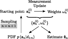

  

  Concept of the classical particle filter

• Measurement update: Calculate the weights $\omega ^{(l)}_{n}$ and determine the posterior PDF $p \left (\mathbf {z}_{n} | d_{1:n}\right)$ (see (56) and (55), respectively).

• Time update: Replace all particles by L new samples drawn from the posterior PDF [30]

  $$\begin{array}{*{20}l} p \left(\mathbf{z}_{n+1} | d_{1:n}\right) = \sum\limits_{l=1}^{L} \omega^{(l)}_{n} p \left(\mathbf{z}_{n+1} | \mathbf{z}^{(l)}_{n}\right), \end{array} $$

  ((58))

  which is equivalent to sampling from $p \left (\mathbf {z}_{n} | d_{1:n}\right)$ and subsequently adding one realization of the uncertainty w _n+1 defined in (10)¹. This is the starting point for the next iteration step.

Unfortunately, the classical particle filter (initially proposed for tracking applications) is conceptually ill-suited for the task of nonlinear AEC: it is well known that the performance degrades with increasing search space and that the local optimization problem is solved without generalizing the instantaneous solution (see the weight calculation in (56)) [41–43]. These properties of the classical particle filter are severe limitations for the task of nonlinear AEC with its high-dimensional state vector (see (22)). To cope with these conceptional limitations without introducing sophisticated resampling methods [40, 44], the elitist particle filter based on evolutionary strategies (EPFES) has been recently proposed in [9]. As major modifications for the task of nonlinear AEC, an evolutionary selection process facilitates to evaluate realizations of the state vector based on recursively calculated particle weights to generalize the instantaneous solution of the optimization problem [9]. These fundamental properties of the EPFES will be illustrated for the state-space model of (7) in the next part.

EPFES [9]: As first modification with respect to the classical particle filter, the particle weights are recursively calculated

$$ \omega^{(l)}_{n} = \gamma \, \omega^{(l)}_{n-1} + (1-\gamma) \frac{p\left(d_{n}|\mathbf{z}^{(l)}_{n} \right)}{\sum\limits_{l=1}^{L} p\left(d_{n}|\mathbf{z}^{(l)}_{n} \right)}, $$

((59))

where γ is the so-called forgetting factor. Following concepts from the field of evolutionary strategies (ES) [45], we subsequently select Q _n elitist particles $\boldsymbol {\bar {z}}^{(q_{n})}_{n}$ with weights larger than a threshold ω _th to determine the posterior PDF $p \left (\mathbf {z}_{n} | d_{1:n}\right)$ (and the MMSE estimate $\hat {\mathbf {z}}_{n}$ as its mean vector) by replacing $\left \{\mathbf {z}^{(l)}_{n},\omega ^{(l)}_{n}\right \}$ in (55) by the set of elitist particles and respective weights $\left \{\bar {\mathbf {z}}^{(q_{n})}_{n},\bar {\omega }^{(q_{n})}_{n}\right \}$. Subsequently, L−Q _n new samples drawn from the posterior PDF $p \left (\mathbf {z}_{n} | d_{1:n}\right)$ replace the non-elitist particles and complete the set of particles for realizing the time update. These steps are illustrated in Fig. 9 and can be summarized as follows:

• Starting point: L particles $\mathbf {z}^{(l)}_{n}$ with weights $\mathbf {\omega }^{(l)}_{n-1}$ determined in the previous time step.

  Fig. 9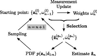

  

  Concept of the EPFES

• Measurement update: Update weights $\omega ^{(l)}_{n}$ in (59), select elitist particles, and determine $p \left (\mathbf {z}_{n} | d_{1:n}\right)$ by inserting the set of elitist particles $\bar {\mathbf {z}}^{(q_{n})}_{n}$ and weights $\bar {\omega }^{(q_{n})}_{n}$ into (55).

• Time update: Replace the non-elitist particles by new samples drawn from the posterior PDF $p \left (\mathbf {z}_{n} | d_{1:n}\right)$. Furthermore, add realizations of w _n+1 (following (7)) to the set of particles (containing Q _n elitist particles and L−Q _n new samples). This is the starting point for the next iteration step².

It has been shown that these modifications of the classical particle filter generalize the instantaneous solution of the optimization problem and thus allow to identify the nonlinear-linear cascade in Fig. 4 [9]. However, the EPFES evaluates realizations of the state vector based on long-term fitness measures. This leads to a high computational complexity due to the high dimension of the state vector in (22). Although many real-time implementations of particle filters have been proposed using parallel processing units [46, 47], it might be necessary for typical applications of nonlinear AEC (e.g., in mobile devices) to reduce the computational complexity to meet specific hardware constraints. Note that a very efficient solution for this problem is the so-called significance-aware EPFES (SA-EPFES) proposed in [19], where the NLMS algorithm (to estimate the linear component of the AEC scenario) is combined with the EPFES (to estimate the loudspeaker signal distortions) by applying significance-aware (SA) filtering. In short, the fundamental idea of SA filtering is to reduce the computational complexity by exploiting physical knowledge about the most significant part of the linear subsystem to estimate the coefficients of the nonlinear preprocessor [18]. Thus, the state vector in (22) underlying the derivation of the SA-EPFES models the coefficients of the nonlinear preprocessor and a small part of the impulse response around the highest energy peak (to capture estimation errors of the NLMS algorithm in the direct-path region).

6 Experimental performance

This overview article establishes a unifying Bayesian network view on linear and nonlinear AEC with the goal to drive future research by highlighting the idealizations and limitations in the probabilistic models of existing methods. Note that a detailed analysis of the adaptive algorithms described in the previous sections has already been performed in [18, 19]. Therefore, we briefly summarize the main findings without explicitly detailing the practical realizations of the algorithms (see [18, 19] for more details). For a recorded female speech signal (commercial smartphone placed on a table with display facing the desk) in a medium-size room with moderate background noise (SNR ≈40 dB), the NLMS algorithm (length-256 FIR filter at 16 kHz) achieved an average echo return loss enhancement (ERLE) of 8.2 dB in a time interval of 9 s [19]. Compared to this, the Hammerstein group model and the SA-EPFES improve the average ERLE by 34 and 68 % at a computational complexity increased by 27 and 50 %, respectively [19]. To achieve these results, the Hammerstein group model (termed as SA-HGM in [18]) and the SA-EPFES are realized based on the concept of SA filtering [18] (11 filter taps for the direct-path region of the RIR) by using length-256 FIR filters and a third-order memoryless preprocessor (inserting odd-order Legendre functions into (18)).

7 Conclusions

In this article, we derived a set of conceptually different algorithms for linear and nonlinear AEC from a unifying graphical model perspective. Based on a concise review of Bayesian networks, we introduced a state-space model with latent state vector capturing all relevant information of the unknown system. After this, we employed three combinations of state-vector definitions (to model a linear or nonlinear echo path) and observation equations (mathematical relation between state vector and observation) to apply fundamental techniques of machine learning research. Thereby, it is shown that the NLMS algorithm, the Hammerstein group model (considered from this perspective here for the first time), and a numerical sampling scheme for nonlinear AEC can be derived from a unifying Bayesian network perspective. This viewpoint highlights probabilistic assumptions underlying different derivations and serves as a basis for developing new algorithms for linear and nonlinear AEC and similar tasks. An example for future work is a Bayesian view on a nonlinear AEC scenario, where the nonlinear loudspeaker signal distortions are modeled by a nonlinear preprocessor with memory.

8 Endnotes

¹ Note that sampling from the posterior PDF $p\left (\mathbf {z}_{n+1} | d_{1:n}\right) \stackrel {(7)}{=} \sum \limits _{l=1}^{L} \omega ^{(l)}_{n} \mathcal {N} \left (\mathbf {z}_{n+1} | \mathbf {z}^{(l)}_{n},C_{\mathbf {w},n+1} \mathbf {I}\right)$ is equivalent to adding samples drawn from the discrete PDF $p \left (\mathbf {z}_{n} | d_{1:n}\right)$ in (55) and the Gaussian PDF $p \left (\mathbf {w}_{n+1}\right)$ in (10).

² In practice, the weights of the new samples for the recursive update in (56) are initialized by the value ω _th.

References

P Dreiseitel, E Hänsler, H Puder, in Proc. Conf. Europ. Signal Process. (EUSIPCO). Acoustic echo and noise control–a long lasting challenge (Rhodes, 1998), pp. 945–952.
E Hänsler, The hands-free telephone problem—an annotated bibliography. Signal Process.27(3), 259–271 (1992).
E Hänsler, in IEEE Int. Symp. Circuits, Systems. The hands-free telephone problem, (1992), pp. 1914–1917.
B Widrow, ME Hoff, in IRE WESCON Conv. Rec. 4. Adaptive switching circuits (Los Angeles, CA, 1960), pp. 96–104.
C Breining, P Dreiseitel, E Hänsler, A Mader, B Nitsch, H Puder, T Schertler, G Schmidt, J Tilp, Acoustic echo control. An application of very-high-order adaptive filters. IEEE Signal Process. Mag.16(4), 42–69 (1999).
E Hänsler, in IEEE Int. Symp. Circuits, Systems. Adaptive echo compensation applied to the hands-free telephone problem (New Orleans, LA, 1990), pp. 279–282.
E Hänsler, G Schmidt, Acoustic Echo and Noise Control: a Practical Approach (J. Wiley and sons, New Jersey, 2004).
A Stenger, W Kellermann, Adaptation of a memoryless preprocessor for nonlinear acoustic echo cancelling. Signal Process.80(9), 1747–1760 (2000).
C Huemmer, C Hofmann, R Maas, A Schwarz, W Kellermann, in Proc. IEEE Int. Conf. Acoustics, Speech, Signal Process. (ICASSP). The elitist particle filter based on evolutionary strategies as novel approach for nonlinear acoustic echo cancellation (Florence, Italy, 2014), pp. 1315–1319.
AN Birkett, RA Goubran, in Proc. IEEE Workshop Neural Networks Signal Process. (NNSP). Nonlinear echo cancellation using a partial adaptive time delay neural network (Cambridge, MA, 1995), pp. 449–458.
LSH Ngja, J Sjobert, in Proc. IEEE Int. Conf. Acoustics, Speech, Signal Process. (ICASSP). Nonlinear acoustic echo cancellation using a Hammerstein model (Seattle, WA, 1998), pp. 1229–1232.
M Zeller, LA Azpicueta-Ruiz, J Arenas-Garcia, W Kellermann, Adaptive Volterra filters with evolutionary quadratic kernels using a combination scheme for memory control. IEEE Trans. Signal Process.59(4), 1449–1464 (2011).
F Küch, W Kellermann, Orthogonalized power filters for nonlinear acoustic echo cancellation. Signal Process.86(6), 1168–1181 (2006).
G Li, C Wen, WX Zheng, Y Chen, Identification of a class of nonlinear autoregressive models with exogenous inputs based on kernel machines. IEEE Trans. Signal Process.59(5), 2146–2159 (2011).
J Kivinen, AJ Smola, RC Williamson, Online learning with kernels. IEEE Trans. Signal Process.52(8), 165–176 (2004).
S Shimauchi, Y Haneda, in Proc. IEEE Int. Workshop Acoustic Signal Enhanc. (IWAENC). Nonlinear Acoustic Echo Cancellation Based on Piecewise Linear Approximation with Amplitude Threshold Decomposition (Aachen, Germany, 2012), pp. 1–4.
S Malik, G Enzner, in Proc. IEEE Int. Conf. Acoustics, Speech, Signal Process. (ICASSP). Variational Bayesian inference for nonlinear acoustic echo cancellation using adaptive cascade modeling (Kyoto, 2012), pp. 37–40.
C Hofmann, C Huemmer, W Kellermann, in Proc. IEEE Int. Conf. Acoustics, Speech, Signal Process. (ICASSP). Significance-aware Hammerstein group models for nonlinear acoustic echo cancellation (Florence, Italy, 2014), pp. 5934–5938.
C Huemmer, C Hofmann, R Maas, W Kellermann, in Proc. IEEE Global Conf. Signal Information Process. (GlobalSIP). The significance-aware EPFES to estimate a memoryless preprocessor for nonlinear acoustic echo cancellation (Atlanta, GA, 2014), pp. 557–561.
T Adali, D Miller, K Diamantaras, J Larsen, Trends in machine learning for signal processing. IEEE Signal Process. Mag.28(6), 193–196 (2011).
R Talmon, I Cohen, S Gannot, RR Coifman, Diffusion maps for signal processing: a deeper look at manifold-learning techniques based on kernels and graphs. IEEE Signal Process. Mag.30(4), 75–86 (2013).
K-R Muller, T Adali, K Fukumizu, JC Principe, S Theodoridis, Special issue on advances in kernel-based learning for signal processing. IEEE Signal Process. Mag.30(4), 14–15 (2013).
BJ Frey, Graphical Models for Machine Learning and Digital Communication (MIT Press, Cambridge, MA, USA, 1998).
SJ Rennie, P Aarabi, BJ Frey, Variational probabilistic speech separation using microphone arrays. IEEE Trans. Audio, Speech, Lang. Process.15(1), 135–149 (2007).
S Malik, J Benesty, J Chen, A Bayesian framework for blind adaptive beamforming. IEEE Trans. Signal Process.62(9), 2370–2384 (2014).
FR Kschischang, BJ Frey, H-A Loeliger, Factor graphs and the sum-product algorithm. IEEE Trans. Inform. Theory. 47(2), 498–519 (2001).
P Mirowski, Y LeCun, in Machine Learning and Knowledge Discovery in Databases, Lecture Notes in Computer Science, 5782. Dynamic factor graphs for time series modeling (Springer,Berlin Heidelberg, 2009), pp. 128–143.
CW Maina, JM Walsh, Joint speech enhancement and speaker identification using approximate Bayesian inference. IEEE Trans. Audio, Speech, Lang. Process.19(6), 1517–1529 (2011).
D Barber, AT Cemgil, Graphical models for time series. IEEE Signal Process. Mag.27(6), 18–28 (2010).
CM Bishop, Pattern Recognition and Machine Learning (Springer, New York, 2006).
R Maas, C Huemmer, C Hofmann, W Kellermann, in ITG Conf. Speech Commun. On Bayesian networks in speech signal processing (Erlangen, Germany, 2014).
C Huemmer, R Maas, W Kellermann, The NLMS algorithm with time-variant optimum stepsize derived from a Bayesian network perspective. IEEE Signal Process. Lett.22(11), 1874–1878 (2015).
PAC Lopes, JB Gerald, in Proc. IEEE Int. Conf. Acoustics, Speech, Signal Process. (ICASSP). New normalized LMS algorithms based on the Kalman filter (New Orleans, LA, 2007), pp. 117–120.
S Yamamoto, S Kitayama, An adaptive echo canceller with variable step gain method. Trans. IECE Japan. E65(1), 1–8 (1982).
S Haykin, Adaptive Filter Theory (Prentice Hall, New Jersey, 2002).
U Schultheiß, Über die adaption eines kompensators für akustische echos. VDI Verlag (1988).
C Breining, P Dreiseitel, E Hänsler, A Mader, B Nitsch, H Puder, T Schertler, G Schmidt, J Tilp, Acoustic echo control. Signal Process.16(4), 42–69 (1999).
R Maas, C Huemmer, A Schwarz, C Hofmann, W Kellermann, in Proc. IEEE China Summit Int. Conf. Signal Information Process. (ChinaSIP). A Bayesian network view on linear and nonlinear acoustic echo cancellation (Xi’an, China, 2014), pp. 495–499.
K Uosaki, T Hatanaka, Nonlinear state estimation by evolution strategies based particle filters. 2003 Congr. Evolut. Comput.3:, 2102–2109 (2003).
T Schön. Estimation of nonlinear dynamic systems (PhD thesis, Linköpings universitetLiU-Tryck, 2006).
T Bengtsson, P Bickel, B Li, in Probability, Statistics: Essays Honor David A. Freedman, Vol. 2. Curse-of-dimensionality revisited: collapse of the particle filter in very large scale systems (Institute of Mathematical StatisticsBeachwood, Ohio, USA, 2008), pp. 316–334.
F Gustafsson, F Gunnarsson, N Bergman, U Forssell, J Jansson, R Karlsson, P-J Nordlund, Particle filters for positioning, navigation, and tracking. IEEE Trans. Signal Process.50(2), 425–437 (2002).
A Doucet, AM Johansen, A tutorial on particle filtering and smoothing: fifteen years later. Handbook Nonlinear Filtering. 12:, 656–704 (2009).
A Doucet, N de Freitas, N Gordon, Sequential Monte Carlo Methods in Practice (Springer, New York, 2001).
T Bäck, H-P Schwefel, in Proc. IEEE Int. Conf. Evolut. Comput. (ICEC). Evolutionary computation: an overview (Nagoya, Japan, 1996), pp. 20–29.
S Henriksen, A Wills, TB T. Schön, B Ninness, in Proc. 16th IFAC Symposium Syst. Ident, 16. Parallel implementation of particle MCMC methods on a GPU (Brussels, Belgium, 2012), pp. 1143–1148.
A Lee, C Yau, MB Giles, A Doucet, CC Holmes, On the utility of graphics cards to perform massively parallel simulation of advanced monte carlo methods. J. Comp. Graph. Stat.19(4), 769–789 (2010).
Acknowledgements
The authors would like to thank the Deutsche Forschungsgemeinschaft (DFG) for supporting this work (contract number KE 890/4-2).
Author information
Authors and Affiliations
Corresponding author
Additional information
Competing interests
The authors declare that they have no competing interests.
Authors’ information
RM was with the University of Erlangen-Nuremberg while the work has been conducted. He is now with Amazon, Seattle, WA.
Rights and permissions
Open Access This article is distributed under the terms of the Creative Commons Attribution 4.0 International License (http://creativecommons.org/licenses/by/4.0/), which permits unrestricted use, distribution, and reproduction in any medium, provided you give appropriate credit to the original author(s) and the source, provide a link to the Creative Commons license, and indicate if changes were made.
About this article
Cite this article
Huemmer, C., Maas, R., Hofmann, C. et al. A Bayesian network approach to linear and nonlinear acoustic echo cancellation. EURASIP J. Adv. Signal Process. 2015, 98 (2015). https://doi.org/10.1186/s13634-015-0282-2
Received:
Accepted:
Published:
DOI: https://doi.org/10.1186/s13634-015-0282-2