Instantly decodable network coding for real-time scalable video broadcast over wireless networks

Abstract

In this paper, we study real-time scalable video broadcast over wireless networks using instantly decodable network coding (IDNC). Such real-time scalable videos have hard deadline and impose a decoding order on the video layers. We first derive the upper bound on the probability that the individual completion times of all receivers meet the deadline. Using this probability, we design two prioritized IDNC algorithms, namely the expanding window IDNC (EW-IDNC) algorithm and the non-overlapping window IDNC (NOW-IDNC) algorithm. These algorithms provide a high level of protection to the most important video layer, namely the base layer, before considering additional video layers, namely the enhancement layers, in coding decisions. Moreover, in these algorithms, we select an appropriate packet combination over a given number of video layers so that these video layers are decoded by the maximum number of receivers before the deadline. We formulate this packet selection problem as a two-stage maximal clique selection problem over an IDNC graph. Simulation results over a real scalable video sequence show that our proposed EW-IDNC and NOW-IDNC algorithms improve the received video quality compared to the existing IDNC algorithms.

1 Introduction

Network coding has shown great potential to improve throughput, delay, and quality of services in wireless networks [1–10]. These merits of network coding make it an attractive candidate for multimedia applications [7–9]. In this paper, we are interested in utilizing network coding in real-time scalable video applications [11, 12], which compress video frames in the form of one base layer and several enhancement layers. The base layer provides the basic video quality, and the enhancement layers provide successive improved video qualities. Using such a scalable video stream, the sender adapts the video bit rate compatible to the available network bandwidth by sending the base layer and as many enhancement layers as possible. Moreover, the real-time scalable video has two distinct characteristics. First, it has a hard deadline before which the video layers need to be decoded to be usable at the application. Second, the video layers exhibit a hierarchical order such that a video layer can be decoded only if this layer and all its lower layers are received. Even though scalable video can tolerate the loss of one or more enhancement layers, this adversely affects the video quality experienced by viewers. Therefore, it is desirable to design network coding schemes so that the received packets before the deadline contribute to decoding the maximum number of video layers.

Fountain codes such as random linear network codes (RLNC) [13–18], raptor codes [19], and LT codes [20–22] have been studied extensively for efficient data delivery in wireless networks. These codes offer significant performance gains compared to conventional channel codes since channel protection is not pre-determined [21–25]. In case of scalable video transmission, combining the layered approach with fountain codes has shown to further improve the quality of video streaming in [26–30] as it provides unequal error protection to different importance layers. In particular, scalable video delivery from multiple servers to a set of receivers was studied in [26], where each video layer is independently protected by raptor codes. Another work in [27] also studied unequal error protection raptor codes for increasing error robustness of scalable video transmission. The authors in [28] studied expanding window fountain codes for scalable video multicast and illustrated the benefits of using expanding window approaches.

Random linear network coding (RLNC) and instantly decodable network coding (IDNC) have been adopted over LT and raptor codes in many applications and systems [5, 13, 15–18, 31, 32] due to their abilities of simple extension to general networks and providing better trade-offs among bandwidth efficiency, complexity, and delay [7]. The works in [13, 17, 18, 33] designed expanding window-based RLNC strategies for scalable video transmission such that coded packets are formed across different numbers of video layers. In particular, the authors in [17] used a probabilistic approach for selecting coding windows and included the packets in the lower video layers into all coded packets to obtain high decoding probabilities for the lower layers. Moreover, the authors in [18] considered a scalable video transmission with a hard deadline and used a deterministic approach for selecting coding windows over all transmissions before the deadline. Another work in [33] continued the work in [17] and addressed the problem of jointly determining the coding strategy and the scheduling decisions when receivers obtain layered video data from multiple servers. Moreover, a resource-allocation framework for network-coded scalable video multicast services was proposed in [13] that minimizes the number of broadcast packets on each downlink channel while providing service guarantees to a predetermined fraction of receivers.

Our work is inspired by the recent works on scalable video transmission using RLNC in [13, 17, 18, 33]. In this work, we adopt XOR-based instantly decodable network coding (IDNC) to investigate its performance for scalable video transmission. Despite the superior throughput performance of RLNC, IDNC has drawn significant attention due to the following attractive properties. IDNC aims to provide instant packet decodability upon successful packet reception at the receivers. This instant decodability property allows a progressive recovery of the video layers as the receivers decode more packets. Furthermore, the encoding process of IDNC is performed using simple XOR operations compared to the more complicated operations over large Galois fields performed in RLNC. The decoding process of IDNC is also performed using XOR operations, which is suitable for implementation in simple and cost-efficient receivers, compared to complex matrix inversion performed in RLNC [1, 8].

In addition to the inherent simplicity, the throughput performance of IDNC closely follows that of RLNC in a network with a small number of receivers [34]. In particular, IDNC schemes can achieve the optimal throughput for the two-receiver or three-receiver system as shown in [5, 31]. Moreover, as video streaming applications continue to proliferate, the wireless sender often needs to support multiple simultaneously running applications with heterogenous video characteristics. It is well understood that mixing different video sequences can improve video quality in wireless networks [8, 35]. Therefore, the sender can adopt IDNC to encode packets from different video sequences together. This allows immediate decoding of received packets of different video sequences and immediate use of decoded packets at the applications, especially when one or more video sequences are encoded using, for example, multiple description coding in addition to scalable video coding. Such benefits of using IDNC in multiple unicast services was shown in [8, 34, 35].

Another potential application of IDNC-based transmission is sensor networks. In general, sensors are capable of performing limited computational operations and XOR-based decoding operations are readily implementable on small sensors. Imagine a group of sensors that need to execute a set of order-constrained instructions within a fixed amount of time to achieve a desired goal. In other words, there is a hierarchy of instructions that also have a deadline such that the instructions can be executed if previous instructions are executed and they are received before the deadline. Indeed, this problem is equivalent to the problem of interest in this paper, i.e., decoding hierarchical video layers before the deadline.

Due to the aforementioned attractive properties, the authors in [31, 32, 36, 37] considered IDNC for wireless broadcast of a set of packets and aimed to serve the maximum number of receivers with a new packet in each transmission. In [34, 38], the authors addressed the problem of minimizing the number of transmissions required for broadcasting a set of packets in IDNC systems and formulated the problem into a stochastic shortest path (SSP) framework. However, the works in [31, 32, 34, 36–38] neither considered dependency between source packets as is present in the scalable video applications nor considered explicit packet delivery deadline. Several other works in IDNC considered different importance of packets and prioritized packets differently in coding decisions. In particular, the authors in [5] adopted IDNC for video streaming and showed that their proposed IDNC schemes are asymptotically throughput optimal for the three-receiver system subject to sequential packet delivery deadline constraints. However, the work in [5] neither considered dependency between source packets nor considered an arbitrary number of receivers. Another work [8] considered a single layer video transmission and determined the importance of each video packet based on its contribution to the video quality. The selected IDNC packet in [8] maximizes the video quality in the current transmission without taking into account the coding opportunities and the video quality over the successor transmissions before the deadline.

In the context of IDNC for scalable video with multiple layers, the most related works to ours are [39, 40]. In [39], the authors considered that a set of packets forming the base layer has higher priority compared to another set of packets forming the enhancement layers. However, the authors aimed to reduce the number of transmissions required for delivering all the packets instead of reducing the number of transmissions required for delivering the high priority packets. The coding decisions in [39] also searched for the existence of a special IDNC packet that can simultaneously reduce the number of transmissions required for delivering the high priority packets and the number of transmissions required for delivering all the packets. On the other hand, the authors in [40] discussed the hierarchical order of video layers with motivating examples and proposed a heuristic packet selection algorithm. The IDNC algorithm in [40] aimed to balance between the number of transmissions required for delivering the base layer and the number of transmissions required for delivering all video layers. Both works in [39, 40] ignored the hard deadline and did not strictly prioritize to deliver the base layer packets before the deadline. However, for real-time scalable video transmission, addressing the hard deadline for the base layer packets is essential as all other packets depend on the base layer packets.

In this paper, inspired by the real-time scalable video that has a hard deadline and decoding dependency between video layers, we are interested in designing an efficient IDNC framework that maximizes the minimum number of decoded video layers over all receivers before the deadline (i.e., improves fairness in terms of the minimum video quality across all receivers). We consider that the service provider adopts a maxmin policy to improve fairness in terms of the minimum video quality across all receivers regardless of their channel conditions. With such a policy, some receivers experiencing harsh channel conditions are prioritized over other receivers experiencing good channel conditions in order to deliver an acceptable video quality to all revivers. This prevents a severe degradation to the quality of services of a receiver. In such scenarios, by taking into account the deadline, the coding decisions need to carefully balance coding only from the base layer versus coding from all video layers. While the former guarantees the highest level of protection to the base layer, the latter increases the possibility of decoding a large number of video layers before the deadline. In this context, our main contributions are summarized as follows:

• We derive the upper bound on the probability that the individual completion times of all receivers for a given number of video layers meet the deadline. Using this probability, we are able to approximately determine whether the broadcast of a given number of video layers can be completed before the deadline with a predefined probability.

• We design two prioritized IDNC algorithms for scalable video, namely the expanding window IDNC (EW-IDNC) algorithm and the non-overlapping window IDNC (NOW-IDNC) algorithm. EW-IDNC algorithm selects a packet combination over the first video layer and computes the resulting upper bound on the probability that the broadcast of that video layer can be completed before the deadline. Only when this probability meets a predefined high threshold, the algorithm considers additional video layers in coding decisions in order to increase the number of decoded video layers at the receivers. In contrast, NOW-IDNC algorithm always selects a packet combination over the first video layer without exploiting the coding opportunities by including additional video layers.

• In EW-IDNC and NOW-IDNC algorithms, we select an appropriate packet combination over a given number of video layers that increases the possibility of decoding those video layers by the maximum number of receivers before the deadline. We formulate this problem as a two-stage maximal clique selection problem over an IDNC graph. However, the formulated maximal clique selection problem is NP-hard and even hard to approximate. Therefore, we exploit the properties of the problem formulation and design a computationally simple heuristic packet selection algorithm.

• We use a real scalable video sequence to evaluate the performance of our proposed algorithms. Simulation results show that our proposed EW-IDNC and NOW-IDNC algorithms increase the minimum number of decoded video layers over all receivers compared to the IDNC algorithms in [32, 40] and achieve a comparable performance compared to the expanding window RLNC algorithm in [17, 18] while preserving the benefits of IDNC strategies.

• To reduce the feedback load of a network, we extend our proposed IDNC framework for a perfect feedback scenario to an intermittent feedback scenario, where the receivers send feedback after several time slots and the feedback are subject to erasures.

The rest of this paper is organized as follows. The system model and IDNC graph are described in Section 2. We illustrate the importance of appropriately choosing a coding window in Section 3 and draw several guidelines for prioritized IDNC algorithms in Section 4. Using these guidelines, we design two prioritized IDNC algorithms in Section 5. We formulate the problem of finding an appropriate packet combination in Section 6 and design a heuristic packet selection algorithm in Section 7. Simulation results are presented in Section 8. Our proposed IDNC framework is extended to an intermittent feedback scenario in Section 9. Finally, Section 10 concludes the paper.

2 Scalable video broadcast system

2.1 Scalable video coding

We consider a system that employs the scalable video codec (SVC) extension to H.264/AVC video compression standard [11, 12]. A group of pictures (GOP) in scalable video has several video layers and the information bits of each video layer is divided into one or more packets. The video layers exhibit a hierarchical order such that each video layer can only be decoded after successfully receiving all the packets of this layer and its lower layers. The first video layer (known as the base layer) encodes the lowest temporal, spatial, and quality levels of the original video, and the successor video layers (known as the enhancement layers) encode the difference between the video layers of higher temporal, spatial, and quality levels and the base layer. With the increase in the number of decoded video layers, the video quality improves at the receivers.

2.2 System model

We consider a wireless sender (e.g., a base station or a wireless access point) that wants to broadcast a set of N source packets forming a GOP, $\mathcal {N} = \{P_{1},\ldots,P_{N}\}$, to a set of M receivers, $\mathcal {M} = \{R_{1},\ldots,R_{M}\}$. Throughout this paper, we use calligraphic letters to denote sets and their corresponding capital letters to denote the cardinalities of these sets (e.g., $N = |\mathcal N|$). A network coding scheme is applied on the packets of a single GOP as soon as all the packets are ready, which implies that neither merging of GOPs nor buffering of packets in more than one GOP at the sender is allowed. This significant aspect arises from the minimum delivery delay requirement in real-time video streaming. Time is slotted and the sender can transmit one packet per time slot t. There is a limit on the total number of allowable time slots Θ used to broadcast the N packets to the M receivers, as the deadline for the current GOP expires after Θ time slots. Therefore, at any time slot t∈ [1,2,…,Θ], the sender can compute the number of remaining transmissions for the current GOP as, Q=Θ−t+1.

In this paper, we consider that the receivers access the shared channel using time division multiple access (TDMA) protocol. At any time slot t, the portion of time allocated to receiver R _i is denoted by ${x_{t}^{i}}$, and the allocations of time to all receivers satisfy the constraint $\sum _{R_{i} \in \mathcal M} {x_{t}^{i}} \leq 1$. Note that the work in [41] considered a similar TDMA protocol and the works in [13, 14] considered an orthogonal frequency-division multiple access (OFDMA) protocol in designing random linear network coded systems.

In the scalable video broadcast system, the sender has L scalable video layers and each video layer consists of one or more packets. Let set $\mathcal {N} = \{{P_{1}^{1}}\ldots P_{n_{1}}^{1},\ldots,{P_{1}^{L}}\ldots P_{n_{L}}^{L}\}$ denotes all the packets in the L video layers, with n _ℓ being the number of packets in the ℓth video layer. In fact, $N = \sum _{\ell =1}^{L} n_{\ell }$. Although the number of video layers in a GOP of a video stream is fixed, depending on the video content, n _ℓ and N can have different values for different GOPs. We denote the set that contains all packets in the first ℓ video layers as $\mathcal {N}^{1:\ell }$ and the cardinality of $\mathcal {N}^{1:\ell }$ as N ^1:ℓ.

The receivers are assumed to be heterogeneous (i.e., the channels between the sender and the receivers are independent but not necessarily identical), and each transmitted packet is subject to an independent Bernoulli erasure at receiver R _i with probability ε _i . Each receiver listens to all transmitted packets and feeds back to the sender a positive or negative acknowledgement (ACK or NAK) for each received or lost packet. We assume that the receivers send feedback to the sender using dedicated control channels and the feedback is error-free. A stronger channel error correcting code is often employed for control bits compared to the data bits. Moreover, the feedback transmission from the receivers to the sender experiences a low interference level since the sender (e.g., base station) is located at the center of a cell. Note that a receiver needs to use γ bits for a rate $\frac {1}{\gamma }$ error correction code to acknowledge a received/lost packet. Since there are M receivers in the network, the overall communication overhead coming from feedback is γ×M bits per time slot. Indeed, the feedback messages require additional resources from a cellular network. To reduce the feedback load, the number of feedback messages can be scaled down with the increased number of receivers in the network. Consequently, we extend our proposed IDNC framework for a perfect feedback scenario to an intermittent feedback scenario in Section 9, where the receivers send feedback after several time slots and the feedback is subject to erasures.

After each transmission, the sender stores the reception status of all packets at all receivers in an M×N state feedback matrix (SFM) $\mathbf {F} = \,[f_{i,j}], \; \forall R_{i} \in \mathcal {M}, P_{j}\in \mathcal {N}$ such that:

$$ f_{i,j} = \left\{\begin{array}{cc} 0 & \text{if packet \(P_{j}\) is received by receiver \(R_{i}\)}, \\ 1 & \text{if packet \(P_{j}\) is missing at receiver \(R_{i}\)}. \end{array}\right. $$

((1))

Example 1.

An example of SFM with M=2 receivers and N=5 packets is given as follows:

$$ \mathbf{F} = \left(\begin{array}{ccccc} 1 & 0 & 1 & 1 & 1\\ 0 & 1 & 1 & 0 & 0\\ \end{array}\right). $$

((2))

In this example, we assume that packets P ₁ and P ₂ belong to the first (i.e., base) layer, packets P ₃ and P ₄ belong to the second layer and packet P ₅ belongs to the third layer. Therefore, the set containing all packets in the first two video layers is $\mathcal {N}^{1:2} =\{P_{1},P_{2},P_{3},P_{4}\}$.

Definition 1.

A window over the first ℓ video layers (denoted by ω _ℓ ) includes all the packets in $\mathcal {N}^{1:\ell } = \{{P_{1}^{1}},{P_{2}^{1}},\ldots,P_{n_{1}}^{1},\ldots,P_{1}^{\ell },P_{2}^{\ell },\ldots,P_{n_{\ell }}^{\ell } \}$.

There are L windows for a GOP with L video layers as shown in Fig. 1. The SFM corresponding to the window ω _ℓ over the first ℓ video layers is an M×N ^1:ℓ matrix F ^1:ℓ, which contains the first N ^1:ℓ columns of SFM F.

Fig. 1

L windows for an L-layer GOP with n _ℓ packets in the ℓth layer

Based on the SFM, the following two sets of packets can be attributed to each receiver R _i at any given time slot t:

• The Has set of receiver R _i in the first ℓ video layers ($\mathcal {H}_{i}^{1:\ell }$) is defined as the set of packets that are decoded by receiver R _i from the first ℓ video layers. In Example 1, the Has set of receiver R ₂ in the first two video layers is $\mathcal {H}_{2}^{1:2} = \{P_{1}, P_{4}\}$.

• The Wants set of receiver R _i in the first ℓ video layers ($\mathcal {W}_{i}^{1:\ell }$) is defined as the set of packets that are missing at receiver R _i from the first ℓ video layers. In other words, $\mathcal {W}_{i}^{1:\ell } = \mathcal {N}^{1:\ell } \setminus \mathcal {H}_{i}^{1:\ell }$. In Example 1, the Wants set of receiver R ₂ in the first two video layers is $\mathcal {W}_{2}^{1:2} = \{P_{2}, P_{3}\}$.

The cardinalities of $\mathcal {H}_{i}^{1:\ell }$ and $\mathcal {W}_{i}^{1:\ell }$ are denoted by $H_{i}^{1:\ell }$ and $W_{i}^{1:\ell }$, respectively. The set of receivers having non-empty Wants sets in the first ℓ video layers is denoted by $\mathcal M_{w}^{1:\ell }$ (i.e., $\mathcal {M}_{w}^{1:\ell } = \left \{R_{i} \middle | \mathcal {W}_{i}^{1:\ell } \neq \varnothing \right \}$). At any given SFM F ^1:ℓ at time slot t, receiver R _i having non-empty Wants set in the first ℓ video layers $\left (i.e., R_{i} \in \mathcal {M}_{w}^{1:\ell }\right)$ belongs to one of the following three sets:

• The critical set of receivers for the first ℓ video layers ($\mathcal {C}^{1:\ell }$) is defined as the set of receivers with the number of missing packets in the first ℓ video layers being equal to the number of remaining Q transmissions $\left (i.e., W_{i}^{1:\ell } = Q, \forall R_{i} \in \mathcal {C}^{1:\ell }\right)$.

• The affected set of receivers for the first ℓ video layers ($\mathcal {A}^{1:\ell }$) is defined as the set of receivers with the number of missing packets in the first ℓ video layers being greater than the number of remaining Q transmissions $\left (i.e., W_{i}^{1:\ell } > Q, \forall R_{i} \in \mathcal {A}^{1:\ell }\right)$.

• The non-critical set of receivers for the first ℓ video layers ($\mathcal {B}^{1:\ell }$) is defined as the set of receivers with the number of missing packets in the first ℓ video layers being less than the number of remaining Q transmissions $\left (i.e., W_{i}^{1:\ell } < Q, \forall R_{i} \in \mathcal {B}^{1:\ell }\right)$.

In fact, $\mathcal {C}^{1:\ell } \cup \mathcal {A}^{1:\ell } \cup \mathcal {B}^{1:\ell } = \mathcal {M}_{w}^{1:\ell }$. We denote the cardinalities of $\mathcal {C}^{1:\ell }$, $\mathcal {A}^{1:\ell }$, and $\mathcal {B}^{1:\ell }$ as C ^1:ℓ, A ^1:ℓ, and B ^1:ℓ, respectively.

Definition 2.

A transmitted packet is instantly decodable for receiver R _i if it contains exactly one source packet from $\mathcal {W}_{i}^{1:L}$.

Definition 3.

Receiver R _i is targeted by packet P _j in a transmission when this receiver will immediately decode missing packet P _j upon successfully receiving the transmitted packet.

Definition 4.

At time slot t, individual completion time of receiver R _i for the first ℓ video layers (denoted by $T_{W_{i}^{1:\ell }}$) is the total number of transmissions required to deliver all the missing packets in $\mathcal {W}_{i}^{1:\ell }$ to receiver R _i .

Individual completion time of receiver R _i for the first ℓ video layers can be $T_{W_{i}^{1:\ell }} = W_{i}^{1:\ell }, W_{i}^{1:\ell }+1,...$ depending on the number of transmissions that receiver R _i is targeted with a new packet and the channel erasures experienced by receiver R _i in those transmissions.

Definition 5.

At time slot t, individual completion times of all receivers for the first ℓ video layers (denoted by T ^1:ℓ) is the total number of transmissions required to deliver all the missing packets from the first ℓ video layers to all receivers in $\mathcal M_{w}^{1:\ell }$.

Definition 6.

At time slot t, individual completion times of all non-critical receivers for the first ℓ video layers (denoted by $T_{B}^{1:\ell }$) is the total number of transmissions required to deliver all the missing packets from the first ℓ video layers to all non-critical receivers in $\mathcal B^{1:\ell }$.

2.3 IDNC graph and packet generation

We define the representation of all feasible packet combinations that are instantly decodable by a subset of, or all receivers, in the form of a graph. As described in [34, 37], the IDNC graph $\mathcal G(\mathcal V, \mathcal E)$ is constructed by first inducing a vertex $v_{\textit {ij}} \in \mathcal V$ for each missing packet $P_{j}\in \mathcal {W}_{i}^{1:L}, \; \forall R_{i}\in \mathcal {M}$. Two vertices v _ij and v _mn in $\mathcal {G}$ are connected (adjacent) by an edge $e_{ij,mn}\in \mathcal E$, when one of the following two conditions holds:

• C1: P _j =P _n , the two vertices are induced by the same missing packet P _j of two different receivers R _i and R _m .

• C2: $P_{j}\in \mathcal {H}_{m}^{1:L}$ and $P_{n}\in \mathcal {H}_{i}^{1:L}$, the requested packet of each vertex is in the Has set of the receiver of the other vertex.

Definition 7.

In an undirected graph, all vertices in a clique are connected to each other with edges. A clique is maximal if it is not a subset of any larger clique [42].

Given this graph representation, the set of all feasible IDNC packets can be defined by the set of all maximal cliques in graph $\mathcal {G}$. The sender can generate an IDNC packet for a given transmission by XORing all the source packets identified by the vertices of a selected maximal clique (denoted by κ) in graph $\mathcal G$. Note that each receiver can have at most one vertex (i.e., one missing packet) in a maximal clique κ and the selection of a maximal clique κ is equivalent to the selection of a set of targeted receivers (denoted by $\mathcal {X}(\kappa)$). A summary of the main notations used in this paper is presented in Table 1.

Table 1 Main notations and their descriptions

3 Importance of appropriately choosing a coding window

In scalable video with multiple layers, the sender needs to choose a window of video layers and the corresponding SFM to select a packet combination in each transmission. In general, different windows lead to different packet combinations and result in different probabilities of completing the broadcast of different numbers of video layers before the deadline. To further illustrate, let us consider the following SFM with M=2 receivers and N=2 packets at time slot t:

$$ \mathbf{F} = \left(\begin{array}{cc} 0 & 1 \\ 1 & 1 \\ \end{array}\right). $$

((3))

In this scenario, we assume that packet P ₁ belongs to the first video layer and packet P ₂ belongs to the second video layer. We further assume that there are two remaining transmissions before the deadline, i.e., Q=2. Given two video layers, there are two windows such as ω ₁={P ₁} and ω ₂={P ₁,P ₂}. With these windows, the possible packet transmissions at time slot t are as follows:

• Case 1: Window ω ₁ leads to packet P ₁ transmission since it targets receiver R ₂ and $\mathcal M_{w}^{1:1} = \{R_{2}\}$.

• Case 2: Window ω ₂ leads to packet P ₂ transmission since it targets receivers R ₁ and R ₂ and $\mathcal M_{w}^{1:2} = \{R_{1}, R_{2}\}$.

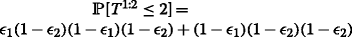
(Case 1:) With packet P ₁ transmitted at time slot t, we can compute the probabilities of completing the broadcast of different numbers of video layers before the deadline as follows.

• The probability of completing the first video layer broadcast before the deadline can be computed as, . Here, (1−ε ₂) defines the packet reception probability at receiver R ₂ at time slot t and ε ₂(1−ε ₂) defines the probability that packet P ₁ is lost at receiver R ₂ at time slot t and is received at receiver R ₂ at time slot t+1.

  Remark 1. It can be stated that the missing packets of all receivers need to be attempted at least once in order to have a possibility of delivering all the missing packets to all receivers.

• Using Remark 1, the sender transmits packet P ₂ at time slot t+1. Consequently, the probability of completing both video layers’ broadcast before the deadline can be computed as, . This is the probability that each missing packet is received in the first attempt.

A summary of probability expressions used for Case 1 can be found in Table 2.

Table 2 Probability expressions used in Case 1, where packet P ₁ is transmitted at time slot t. With this transmission, the first layer completion probability before the deadline and both layers’ completion probability before the deadline are shown

(Case 2:) With packet P ₂ transmitted at time slot t, we can compute the probabilities of completing the broadcast of different numbers of video layers before the deadline as follows.

• The sender transmits packet P ₁ at time slot t+1. Consequently, the probability of completing the first video layer broadcast before the deadline can be computed as, . This is the probability that packet P ₁ is received at receiver R ₂ at time slot t+1.

• Using Remark 1, the sender transmits either coded packet P ₁⊕P ₂ or packet P ₁ at time slot t+1. Consequently, the probability of completing both video layers’ broadcast before the deadline can be computed as, .

  • ε ₁(1−ε ₂)(1−ε ₁)(1−ε ₂) represents coded packet P ₁⊕P ₂ transmission at time slot t+1. The transmitted packet P ₂ at time slot t can be lost at receiver R ₁ with probability ε ₁ and can be received at receiver R ₂ with probability (1−ε ₂). With this loss and reception status, the sender transmits coded packet P ₁⊕P ₂ to target both receivers and the probability that both receivers receive the transmitted packet is (1−ε ₁)(1−ε ₂).

  • (1−ε ₁)(1−ε ₂)(1−ε ₂) represents packet P ₁ transmission at time slot t+1. This is the probability that each missing packet is received in the first attempt.

A summary of probability expressions used for Case 2 can be found in Table 3. Using the results in Case 1 and Case 2, we conclude for the given time slot t the following:

• Packet P ₁ transmission resulting from window ω ₁ is a better decision in terms of completing the first video layer broadcast since is larger in Case 1.

  Table 3 Probability expressions used in Case 2, where packet P ₂ is transmitted at time slot t. With this transmission, the first layer completion probability before the deadline 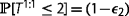and both layers’ completion probability before the deadline are shown

• Packet P ₂ transmission resulting from window ω ₂ is a better decision in terms of completing both video layers broadcast since is larger in Case 2.

Remark 2.

The above example illustrates that it is not always possible to select a packet combination that achieves high probabilities of completing the broadcast of different numbers of video layers before the deadline. In general, some packet transmissions (resulting from different windows) can increase the probability of completing the broadcast of the first video layer, but reduce the probability of completing the broadcast of all video layers and vice versa.

4 Guidelines for prioritized IDNC algorithms

In this section, we first show that finding the optimal IDNC schedule that maximizes the minimum number of decoded video layers over all receivers before the deadline is computationally complex. We then systematically draw several guidelines for the prioritized IDNC algorithms that efficiently increase the minimum number of decoded video layers over all receivers before the deadline.

4.1 Maximizing the minimum decoded video layers problem formulation

Definition 8.

A transmission schedule $\mathcal S = \{\kappa (t)\}, \forall t \in \{1,\ldots,\Theta \}$ is defined as the set of packet combinations at every time slot t before the deadline. Furthermore, S is the set of all possible transmission schedules and $\mathcal S \in \mathbf {S}$.

Definition 9.

The individual decoded video layer $e_{i}(\mathcal S)$ of receiver R _i is defined as the number of decoded video layers at receiver R _i at the end of the deadline for a given transmission schedule $\mathcal S$. Here, individual decoded video layer $e_{i}(\mathcal S)$ of receiver R _i can be {1,…,L}.

For a given transmission schedule $\mathcal S$ and packet reception probabilities of the targeted receivers in schedule $\mathcal S$, the sender can compute the expected number of individual decoded video layer of each receiver. We now define the problem of maximizing the minimum number of decoded video layers over all receivers before the deadline as a transmission schedule selection problem such that:

((4))

The optimization problem in (4) can be formulated into a finite horizon Markov decision process framework and the optimal transmission schedule can be found using the backward induction algorithm, which is a dynamic programming approach. However, the works in [34, 38] showed that finding the optimal IDNC schedule for wireless broadcast of a set of packets is computationally intractable due to the curse of dimensionality of the dynamic programming approach. Therefore, to efficiently solve the optimization problem in (4) with much lower computational complexity, we draw several guidelines for the prioritized IDNC algorithms in the following three subsections.

4.2 Feasible windows of video layers

For a given SFM F at time slot t, we now determine the video layers which can be included in a feasible window and can be considered in coding decisions.

Definition 10.

The smallest feasible window (i.e., window ω _ℓ ) includes the minimum number of successive video layers such that the Wants set of at least one receiver in those video layers is non-empty. This can be defined as, ω _ℓ = min{|ω ₁|,…,|ω _L |} such that $\exists R_{i} | \mathcal W_{i}^{1:\ell } \neq \varnothing$.

In this paper, we address the problem of maximizing the minimum number of decoded video layers over all receivers. Therefore, we define the largest feasible window as follows:

Definition 11.

The largest feasible window (i.e., window ω _ℓ+μ , where μ can be 0,1,…,L−ℓ) includes the maximum number of successive video layers such that the Wants sets of all receivers in those video layers are less than or equal to the remaining Q transmissions. This can be defined as, ω _ℓ+μ = max{|ω ₁|,…,|ω _L |} such that $\mathcal W_{i}^{1:\ell +\mu } \leq Q, \forall R_{i} \in \mathcal M$.

Note that there is no affected receiver over the largest feasible window ω _ℓ+μ (i.e., all receivers belong to critical and non-critical sets for the first ℓ+μ video layers). In fact, an affected receiver will definitely not be able to decode all its missing packets in the remaining Q transmissions. An exception to considering no affected receiver in the largest feasible window is when it is the smallest feasible window, i.e., ω _ℓ+μ =ω _ℓ , in which case it is possible to have $\mathcal {A}^{1:\ell } (t) \neq \varnothing$.

Definition 12.

A feasible window includes any number of successive video layers ranging from the smallest feasible window ω _ℓ to the largest feasible window ω _ℓ+μ . In other words, a feasible window can be any window from {ω _ℓ ,ω _ℓ+1,…,ω _ℓ+μ }.

Example 2.

To further illustrate the feasible windows, consider the following SFM at time slot t:

$$ \mathbf{F} = \left(\begin{array}{cccccc} 0 & 0 & 1 & 1 & 1 & 1\\ 0 & 0 & 1 & 0 & 0 & 1\\ \end{array}\right). $$

((5))

In this example, we assume that packets P ₁ and P ₂ belong to the first video layer, packets P ₃ and P ₄ belong to the second video layer, packet P ₅ belongs to the third video layer and packet P ₆ belongs to the fourth video layer. We also assume that the number of remaining transmissions Q is equal to 3. The smallest feasible window includes the first two video layers (i.e., ω ₂={P ₁,P ₂,P ₃,P ₄}) and the largest feasible window includes the first three video layers (i.e., ω ₃={P ₁,P ₂,P ₃,P ₄,P ₅}). Note that the fourth video layer is not included in the largest feasible window since receiver R ₁ has three missing packets in the first three layers ($\mathcal W_{1}^{1:3} =\{P_{3},P_{4},P_{5}\}$), which is already equal to the number of remaining three transmissions ($W_{1}^{1:3} = Q = 3$). Figure 2 shows the extracted SFMs from SFM in (5) corresponding to the feasible windows.

Fig. 2

SFMs corresponding to the feasible windows in Example 2

4.3 Probability that the individual completion times meet the deadline

With the aim of designing low complexity prioritized IDNC algorithms, after selecting a packet combination over a given feasible window ω _ℓ at time slot t, we compute the resulting upper bound on the probability that the individual completion times of all receivers for the first ℓ video layers is less than or equal to the remaining Q−1 transmissions (denoted by and will be defined in (11)). Since this probability is computed separately for each receiver and ignores the interdependence of receivers’ packet reception captured in the SFM, its computation is simple and does not suffer from the curse of dimensionality as in [34, 38].

To derive probability , we first consider a scenario with one sender and one receiver R _i . Here, individual completion time of this receiver for the first ℓ layers can be $T_{W_{i}^{1:\ell }} = W_{i}^{1:\ell }, W_{i}^{1:\ell }+1,\ldots$. The probability of $T_{W_{i}^{1:\ell }}$ being equal to $W_{i}^{1:\ell } + z, z \in \, [\!0,1,\ldots,Q-W_{i}]$ can be expressed using negative binomial distribution as:

((6))

Consequently, the probability that individual completion time $T_{W_{i}^{1:\ell }}$ of receiver R _i is less than or equal to the remaining Q transmissions can be expressed as:

((7))

We now consider a scenario with one sender and multiple receivers in $\mathcal M_{w}^{1:\ell }$. We assume that all receivers in $\mathcal M_{w}^{1:\ell }$ are targeted with a new packet in each transmission. This is an ideal scenario and defines a lower bound on individual completion time of each receiver. Consequently, we can compute an upper bound on the probability that individual completion time of each receiver meets the deadline. Although this ideal scenario is not likely to occur due to the instant decodability constraint, we can still use this probability upper bound as a metric in designing our computationally simple IDNC algorithms. Having described the ideal scenario with multiple receivers, for a given feasible window ω _ℓ at time slot t, we compute the upper bound on the probability that individual completion times of all receivers for the first ℓ video layers is less than or equal to the remaining Q transmissions as:

((8))

Due to the instant decodability constraint, it may not be possible to target all receivers in $\mathcal M_{w}^{1:\ell }$ with a new packet at time slot t. After selecting a packet combination over a given feasible window ω _ℓ at time slot t, let $\mathcal X$ be the set of targeted receivers and $\mathcal {M}_{w}^{1:\ell } \setminus \mathcal X$ be the set of ignored receivers. We can express the resulting upper bound on the probability that the individual completion times of all receivers for the first ℓ video layers, starting from the successor time slot t+1, is less than or equal to the remaining Q−1 transmissions as:

((9))

• In the first product in expression (9), we compute the probability that a targeted receiver receives its $W_{i}^{1:\ell }-1$ or $W_{i}^{1:\ell }$ missing packets in the remaining Q−1 transmissions. Note that the number of missing packets at a targeted receiver can be $W_{i}^{1:\ell } -1$ with its packet reception probability (1−ε _i ) or can be $W_{i}^{1:\ell }$ with its channel erasure probability ε _i .

• In the second product in expression (9), we compute the probability that an ignored receiver receives its $W_{i}^{1:\ell }$ missing packets in the remaining Q−1 transmissions.

By taking expectation of packet reception and loss cases in the first product in (9), we can simplify expression (9) as:

((10))

Note that a critical and ignored receiver $R_{i} \in \{\mathcal {C}^{1:\ell } \cap (\mathcal {M}_{w}^{1:\ell } \setminus \mathcal {X})\}$ cannot decode all missing packets in $W_{i}^{1:\ell }$ in the remaining Q−1 transmissions since $W_{i}^{1:\ell }$ is already equal to Q transmissions for a critical receiver. With this remark and an exceptional case of having affected receivers described in Section 4.2, we can set:

((11))

In this paper, we use expression (11) as a metric in designing computationally simple IDNC algorithms for real-time scalable video.

4.4 Design criterion for prioritized IDNC algorithms

In Section 3, we showed that some windows and subsequent packet transmissions increase the probability of completing the broadcast of the first video layer, but reduce the probability of completing the broadcast of all video layers and vice versa. This complicated interplay of selecting an appropriate window motivates us to define a design criterion. The objective of the design criterion is to expand the coding window over the successor video layers (resulting in an increased possibility of completing the broadcast of those video layers) after providing a certain level of protection to the lower video layers.

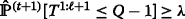
Design Criterion 1.

The design criterion for the first ℓ video layers is defined as the probability meets a certain threshold λ after selecting a packet combination at time slot t.

In other words, the design criterion for the first ℓ video layers is satisfied when logical condition is true after selecting a packet combination at time slot t. Here, probability is computed using expression (11) and threshold λ is chosen according to the level of protection desired for each video layer. In scalable video applications, each decoded layer contributes to the video quality and the layers are decoded following the hierarchical order. Therefore, the selected packet combination at time slot t requires to satisfy the design criterion following the decoding order of the video layers. In other words, the first priority is satisfying the design criterion for the first video layer (i.e., ), the second priority is satisfying the design criterion for the first two video layers (i.e., ) and so on. Having satisfied such a prioritized design criterion, the coding window can continue to expand over the successor video layers to increase the possibility of completing the broadcast of a large number of video layers.

Remark 3.

Threshold λ enables a tradeoff between the mean decoded video layers and the minimum decoded video layers in making decisions in each time slot. In fact, a large threshold value λ (close to 1) results in making a decision over the smallest feasible window and increasing the minimum number of decoded video layers in each time slot. On the other hand, a small threshold value λ (close to 0) results in making a decision over the largest feasible window and increasing the mean number of decoded video layers in each time slot. An intermediate threshold value λ (i.e., 0<λ<1) enables a tradeoff between these two objectives. As a result, the service provider can adopt a threshold value λ based on its prioritized strategies.

5 Prioritized IDNC algorithms for scalable video

In this section, using the guidelines drawn in Section 4, we design two prioritized IDNC algorithms that increase the probability of completing the broadcast of a large number of video layers before the deadline. These algorithms provide unequal levels of protection to the video layers and adopt prioritized IDNC strategies to meet the hard deadline for the most important video layer in each transmission.

5.1 Expanding window instantly decodable network coding (EW-IDNC) algorithm

Our proposed expanding window instantly decodable network coding (EW-IDNC) algorithm starts by selecting a packet combination over the smallest feasible window and iterates by selecting a new packet combination over each expanded feasible window while satisfying the design criterion for the video layers in each window. Moreover, in EW-IDNC algorithm, a packet combination (i.e., a maximal clique κ) over a given feasible window is selected by following methods described in Section 6 or Section 7.

At Step 1 of Iteration 1, the EW-IDNC algorithm selects a maximal clique κ over the smallest feasible window ω _ℓ . At Step 2 of Iteration 1, the algorithm computes the probability using expression (11). At Step 3 of Iteration 1, the algorithm performs one of the following two steps.

• It proceeds to Iteration 2 and considers window and |ω _ℓ |<|ω _ℓ+μ |. This is the case when the design criterion for the first ℓ video layers is satisfied and the window can be further expanded.

• It broadcasts the selected κ at this Iteration 1, if or |ω _ℓ |=|ω _ℓ+μ |. This is the case when the design criterion for the first ℓ video layers is not satisfied or the window is already the largest feasible window.

At Step 1 of Iteration 2, the EW-IDNC algorithm selects a new maximal clique κ over the expanded feasible window ω _ℓ+1. At Step 2 of Iteration 2, the algorithm computes the probability using expression (11). At Step 3 of Iteration 2, the algorithm performs one of the following three steps.

• It proceeds to Iteration 3 and considers window and |ω _ℓ+1|<|ω _ℓ+μ |. This is the case when the design criterion for the first ℓ+1 video layers is satisfied and the window can be further expanded.

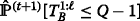
• It broadcasts the selected κ at this Iteration 2, if and |ω _ℓ+1|=|ω _ℓ+μ |. This is the case when the design criterion for the first ℓ+1 video layers is satisfied but the window is already the largest feasible window. Note that when the design criterion for the first ℓ+1 video layers is satisfied, the design criterion for the first ℓ video layers is certainly satisfied since the number of missing packets of any receiver in the first ℓ video layers is smaller than or equal to that in the first ℓ+1 video layers.

• It broadcasts the selected κ at the previous Iteration 1, if . This is the case when the design criterion for the first ℓ+1 video layers is not satisfied.

At Iteration 3, the algorithm performs the steps of Iteration 2. This iterative process is repeated until the algorithm reaches to the largest feasible window ω _ℓ+μ or the design criterion for the video layers over a given feasible window is not satisfied. The proposed EW-IDNC algorithm is summarized in Algorithm 1.

5.2 Non-overlapping window instantly decodable network coding (NOW-IDNC) algorithm

Our proposed non-overlapping window instantly decodable network coding (NOW-IDNC) algorithm always selects a maximal clique κ over the smallest feasible window ω _ℓ by following methods described in Section 6 or Section 7. In fact, this algorithm broadcasts the video layers one after another following their decoding order in a non-overlapping manner. This guarantees the highest level of protection to the most important video layer, which has not yet been decoded by all receivers.

6 Packet selection problem over a given window

In this section, we address the problem of selecting a maximal clique κ over a given window ω _ℓ that increases the possibility of decoding those ℓ video layers by the maximum number of receivers before the deadline. We first extract SFM F ^1:ℓ corresponding to window ω _ℓ and construct IDNC graph $\mathcal G^{1:\ell }$ according to the extracted SFM F ^1:ℓ. We then select a maximal clique κ ^∗ over graph $\mathcal G^{1:\ell }$ in two stages. This approach can be summarized as follows.

• We partition IDNC graph $\mathcal G^{1:\ell }$ into critical graph $\mathcal G_{c}^{1:\ell }$ and non-critical graph $\mathcal G_{b}^{1:\ell }$. The critical graph $\mathcal G_{c}^{1:\ell }$ includes the vertices generated from the missing packets in the first ℓ video layers at the critical receivers in $\mathcal C^{1:\ell }$. Similarly, the non-critical graph $\mathcal G_{b}^{1:\ell }$ includes the vertices generated from the missing packets in the first ℓ video layers at the non-critical receivers in $\mathcal B^{1:\ell }$.

• We prioritize the critical receivers for the first ℓ video layers over the non-critical receivers for the first ℓ video layers since all the missing packets at the critical receivers cannot be delivered without targeting them in the current transmission ($W_{i}^{1:\ell } = Q, \forall R_{i} \in \mathcal C^{1:\ell }$).

• If there is one or more critical receivers (i.e., $\mathcal {C}^{1:\ell } \neq \varnothing$), in the first stage, we select $\kappa _{c}^{*}$ to target a subset of, or if possible, all critical receivers. We define $\mathcal {X}_{c}$ as the set of targeted critical receivers who have vertices in $\kappa _{c}^{*}$.

• If there is one or more non-critical receivers (i.e., $\mathcal {B}^{1:\ell } \neq \varnothing$), in the second stage, we select $\kappa _{b}^{*}$ to target a subset of, or if possible, all non-critical receivers that do not violate the instant decodability constraint for the targeted critical receivers in $\kappa _{c}^{*}$. We define $\mathcal {X}_{b}$ as the set of targeted non-critical receivers who have vertices in $\kappa _{b}^{*}$.

6.1 Maximal clique selection problem over critical graph

With maximal clique $\kappa _{c}^{*}$ selection, each critical receiver in $\mathcal C^{1:\ell }(t)$ experiences one of the following two events at time slot t:

• $R_{i} \in \mathcal {X}_{c}$, the targeted critical receiver can still receive $W_{i}^{1:\ell }$ missing packets in the exact $Q = W_{i}^{1:\ell }$ transmissions.

• $R_{i} \in \mathcal {C}^{1:\ell } \setminus \mathcal {X}_{c}$, the ignored critical receiver cannot receive $W_{i}^{1:\ell }$ missing packets in the remaining Q−1 transmissions and becomes an affected receiver at time slot t+1.

Let $\mathcal {A}^{1:\ell }(t+1)$ be the set of affected receivers for the first ℓ video layers at time slot t+1 after $\kappa _{c}^{*}$ transmission at time slot t. The critical receivers that are not targeted at time slot t will become the new affected receivers, and the critical receivers that are targeted at time slot t can also become the new affected receivers if they experience an erasure in this transmission. Consequently, we can express the expected increase in the number of affected receivers from time slot t to time slot t+1 after selecting $\kappa _{c}^{*}$ as:

((12))

We now formulate the problem of minimizing the expected increase in the number of affected receivers for the first ℓ video layers from time slot t to time slot t+1 as a critical maximal clique selection problem over critical graph $\mathcal G_{c}^{1:\ell }$ such as:

((13))

In other words, the problem of minimizing the expected increase in the number of affected receivers is equivalent to finding all the maximal cliques in the critical IDNC graph, and selecting the maximal clique among them that results in the minimum expected increase in the number of affected receivers.

6.2 Maximal clique selection problem over non-critical graph

Once maximal clique $\kappa _{c}^{*}$ is selected among the critical receivers in $\mathcal {C}^{1:\ell }(t)$, there may exist vertices belonging to the non-critical receivers in non-critical graph $\mathcal G_{b}^{1:\ell }$ that can form even a bigger maximal clique. In fact, if the selected new vertices are connected to all vertices in $\kappa _{c}^{*}$, the corresponding non-critical receivers are targeted without affecting IDNC constraint for the targeted critical receivers in $\kappa _{c}^{*}$. Therefore, we first extract non-critical subgraph $\mathcal G_{b}^{1:\ell }(\kappa _{c}^{*})$ of vertices in $\mathcal G_{b}^{1:\ell }$ that are adjacent to all the vertices in $\kappa _{c}^{*}$ and then select $\kappa _{b}^{*}$ over subgraph $\mathcal {G}_{b}^{1:\ell }(\kappa _{c}^{*})$.

With these considerations, we aim to maximize the upper bound on the probability that individual completion times of all non-critical receivers for the first ℓ video layers, starting from the successor time slot t+1, is less than or equal to the remaining Q−1 transmissions (represented by ). We formulate this problem as a non-critical maximal clique selection problem over graph $\mathcal {G}_{b}^{1:\ell }(\kappa _{c}^{*})$ such as:

((14))

By maximizing probability upon selecting a maximal clique κ _b , the sender increases the probability of transmitting all packets in the first ℓ video layers to all non-critical receivers in $\mathcal B^{1:\ell }(t)$ before the deadline. Using expression (10) for non-critical receivers, we can define expression (14) as:

((15))

In other words, the problem of maximizing probability for all non-critical receivers is equivalent to finding all the maximal cliques in the non-critical subgraph $\mathcal {G}_{b}^{1:\ell }(\kappa _{c}^{*})$ and selecting the maximal clique among them that results in the maximum probability .

Remark 4.

The final maximal clique κ ^∗ over a given window ω _ℓ is the union of two maximal cliques $\kappa _{c}^{*}$ and $\kappa _{b}^{*}$ (i.e., $\kappa ^{*} = \{\kappa _{c}^{*} \cup \kappa _{b}^{*} \}$).

It is well known that a graph with V vertices has O(3^V/3) maximal cliques and finding a maximal clique among them is NP-hard [42]. Therefore, solving the formulated packet selection problem quickly leads to high computational complexity even for systems with moderate numbers of receivers and packets (V=O(M N)). To reduce the computational complexity, it is conventional to design an approximation algorithm. However, the problem is even hard to approximate since there is no O(V ^1−δ) approximation for the best maximal clique among O(3^V/3) maximal cliques for any fixed δ>0 [43].

7 Heuristic packet selection algorithm over a given window

Due to the high computational complexity of the formulated packet selection problem in Section 6, we now design a low-complexity heuristic algorithm following the formulations in (13) and (15). This heuristic algorithm selects maximal cliques κ _c and κ _b based on a greedy vertex search over IDNC graphs $\mathcal G_{c}^{1:\ell }$ and $\mathcal G_{b}^{1:\ell }(\kappa _{c})$, respectively. A similar greedy vertex search approach was studied in [34, 38] due to its computational simplicity. However, the works in [34, 38] solved different problems and ignored the dependency between source packets and the hard deadline. These additional constraints considered in this paper lead us to a different heuristic algorithm with its own features.

• If there is one or more critical receivers (i.e., $\mathcal {C}^{1:\ell }(t) \neq \varnothing$), in the first stage, the algorithm selects maximal clique κ _c to reduce the number of newly affected receivers for the first ℓ video layers after this transmission.

• If there is one or more non-critical receivers (i.e., $\mathcal {B}^{1:\ell }(t) \neq \varnothing$), in the second stage, the algorithm selects maximal clique κ _b to increase the probability after this transmission.

7.1 Greedy maximal clique selection over critical graph

To select critical maximal clique κ _c , the proposed algorithm starts by finding a lower bound on the potential new affected receivers, for the first ℓ video layers from time slot t to time slot t+1, that may result from selecting each vertex from critical IDNC graph $\mathcal G_{c}^{1:\ell }$. At Step 1, the algorithm selects vertex v _ij from graph $\mathcal G_{c}^{1:\ell }$ and adds it to κ _c . Consequently, the lower bound on the expected number of new affected receivers for the first ℓ video layers after this transmission that may result from selecting this vertex can be expressed as:

$$ A^{1:\ell(1)}(t+1) - A^{1:\ell}(t) = C^{1:\ell}(t) - \sum_{R_{m} \in\, \{R_{i} \cup \mathcal M_{ij}^{\mathcal G_{c}^{1:\ell}} \}} (1-\epsilon_{m}). $$

((16))

Here, A ^1:ℓ(1)(t+1) represents the number of affected receivers for the first ℓ video layers at time slot t+1 after transmitting κ _c selected at Step 1 and $\mathcal M_{\textit {ij}}^{\mathcal G_{c}^{1:\ell }}$ is the set of critical receivers that have at least one vertex adjacent to vertex v _ij in $\mathcal G_{c}^{1:\ell }$. Once A ^1:ℓ(1)(t+1)−A ^1:ℓ(t) is calculated for all vertices in $\mathcal G_{c}^{1:\ell }$, the algorithm chooses vertex $v_{\textit {ij}}^{*}$ with the minimum lower bound on the expected number of new affected receivers as:

$$ v_{ij}^{*} = \arg\min_{v_{ij} \in \mathcal G_{c}^{1:\ell}} \left\{A^{1:\ell(1)}(t+1) - A^{1:\ell}(t) \right\}. $$

((17))

After adding vertex $v_{\textit {ij}}^{*}$ to κ _c (i.e., $\kappa _{c} = \{v_{\textit {ij}}^{*} \}$), the algorithm extracts the subgraph $\mathcal G_{c}^{1:\ell }(\kappa _{c})$ of vertices in $\mathcal G_{c}^{1:\ell }$ that are adjacent to all the vertices in κ _c . At Step 2, the algorithm selects another vertex v _mn from subgraph $\mathcal G_{c}^{1:\ell }(\kappa _{c})$ and adds it to κ _c . Consequently, the new lower bound on the expected number of new affected receivers can be expressed as:

$$\begin{array}{*{20}l} &A^{1:\ell(2)}(t+1) - A^{1:\ell}(t) \\ & = C^{1:\ell}(t) - \\ & \;\;\;\;\;\; (\sum_{R_{i} \in \mathcal{X}_{c}(\kappa_{c})} (1-\epsilon_{i}) + \sum_{R_{o} \in \{R_{m} \cup \mathcal M_{mn}^{\mathcal G_{c}^{1:\ell}(\kappa_{c})} \}} (1-\epsilon_{o})) \\ &= (C^{1:\ell}(t) - \sum_{R_{m} \in \{R_{i} \cup \mathcal M_{ij}^{\mathcal G_{c}^{1:\ell}} \}} (1-\epsilon_{m})) + \\ &\;\;\;\;\;\;\;\;\;\;\; \sum_{R_{o} \in \mathcal M_{ij}^{\mathcal G_{c}^{1:\ell}} \setminus (R_{m} \cup \mathcal M_{mn}^{\mathcal G_{c}^{1:\ell}(\kappa_{c})})} (1-\epsilon_{o}) \\ &= (A^{1:\ell(1)}(t+1) - A^{1:\ell}(t)) + \\ & \;\;\;\;\;\;\;\;\;\;\; \sum_{R_{o} \in\, \{ \mathcal M_{ij}^{\mathcal G_{c}^{1:\ell}} \setminus (R_{m} \cup \mathcal M_{mn}^{\mathcal G_{c}^{1:\ell}(\kappa_{c})}) \}} (1-\epsilon_{o}). \end{array} $$

((18))

Since $\left (R_{m} \cup \mathcal M_{\textit {mn}}^{\mathcal G_{c}^{1:\ell }(\kappa _{c})}\right)$ is a subset of $\mathcal M_{\textit {ij}}^{\mathcal G_{c}^{1:\ell }}$, the last term in (18) is resulting from the stepwise increment on the lower bound on the expected number of newly affected receivers due to selecting vertex v _mn . Similar to Step 1, once A ^1:ℓ(2)(t+1)−A ^1:ℓ(t) is calculated for all vertices in the subgraph $\mathcal G_{c}^{1:\ell }(\kappa _{c})$, the algorithm chooses vertex $v_{\textit {mn}}^{*}$ with the minimum lower bound on the expected number of new affected receivers as:

$$ v_{mn}^{*} = \arg\min_{v_{mn} \in \mathcal G_{c}^{1:\ell} (\kappa_{c})} \{A^{1:\ell(2) }(t+1)- A^{1:\ell}(t) \}. $$

((19))

After adding new vertex $v_{\textit {mn}}^{*}$ to κ _c (i.e., $\kappa _{c} = \{\kappa _{c}, v_{\textit {mn}}^{*} \}$), the algorithm repeats the vertex search process until no further vertex in $\mathcal G_{c}^{1:\ell }$ is adjacent to all the vertices in κ _c .

7.2 Greedy maximal clique selection over non-critical graph

To select non-critical maximal clique κ _b , the proposed algorithm extracts the non-critical IDNC subgraph $\mathcal G_{b}^{1:\ell }(\kappa _{c})$ of vertices in $\mathcal G_{b}^{1:\ell }$ that are adjacent to all the vertices in κ _c . This algorithm starts by finding the maximum probability that may result from selecting each vertex from subgraph $\mathcal G_{b}^{1:\ell }(\kappa _{c})$. At Step 1, the algorithm selects vertex v _ij from $\mathcal G_{b}^{1:\ell }(\kappa _{c})$ and adds it to κ _b . Consequently, the probability that may result from selecting this vertex at Step 1 can be computed as:

((20))

Here, $\mathcal M_{\textit {ij}}^{\mathcal G_{b}^{1:\ell }(\kappa _{c})}$ is the set of non-critical receivers that have at least one vertex adjacent to vertex v _ij in $\mathcal G_{b}^{1:\ell }(\kappa _{c})$. Once probability is calculated for all vertices in $\mathcal G_{b}^{1:\ell }(\kappa _{c})$, the algorithm chooses vertex $v_{\textit {ij}}^{*}$ with the maximum probability as:

((21))

After adding vertex $v_{\textit {ij}}^{*}$ to κ _b (i.e., $\kappa _{b} = \{v_{\textit {ij}}^{*} \}$), the algorithm extracts the subgraph $\mathcal G_{b}^{1:\ell }(\kappa _{c} \cup \kappa _{b})$ of vertices in $\mathcal G_{b}^{1:\ell }(\kappa _{c})$ that are adjacent to all the vertices in (κ _c ∪κ _b ). At Step 2, the algorithm selects another vertex v _mn from subgraph $\mathcal G_{b}^{1:\ell }(\kappa _{c} \cup \kappa _{b})$ and adds it to κ _b . Note that the new set of potentially targeted non-critical receivers after Step 2 is $\{R_{i} \cup R_{m} \cup \mathcal M_{\textit {mn}}^{\mathcal G_{b}^{1:\ell }(\kappa _{c} \cup \kappa _{b})}\}$, which is a subset of $\{R_{i} \cup \mathcal M_{\textit {ij}}^{\mathcal G_{b}^{1:\ell }(\kappa _{c})}\}$. Consequently, the new probability due to the stepwise reduction in the number of targeted non-critical receivers can be computed as:

((22))

Similar to Step 1, once probability is calculated for all vertices in the subgraph $\mathcal G_{b}^{1:\ell }(\kappa _{c} \cup \kappa _{b})$, the algorithm chooses vertex $v_{\textit {mn}}^{*}$ with the maximum probability as:

((23))

After adding new vertex $v_{\textit {mn}}^{*}$ to κ _b (i.e., $\kappa _{b} = \{\kappa _{b}, v_{\textit {mn}}^{*} \}$), the algorithm repeats the vertex search process until no further vertex in $\mathcal G_{b}^{1:\ell }$ is adjacent to all the vertices in (κ _c ∪κ _b ). The final maximal clique κ over a given window ω _ℓ is the union of κ _c and κ _b (i.e., κ=κ _c ∪κ _b ). The proposed heuristic algorithm is summarized in Algorithm 2.

Remark 5.

The complexity of the proposed heuristic packet selection algorithm is O(M ² N) since it requires weight computations for the O(M N) vertices in each step and a maximal clique can have at most M vertices. Using this heuristic algorithm, the complexity of the EW-IDNC algorithm is O(M ² N L) since it can perform the heuristic algorithm at most L times over L windows. Moreover, using this heuristic algorithm, the complexity of the NOW-IDNC algorithm is O(M ² N) since it performs the heuristic algorithm once over the smallest feasible window.

8 Simulation results over a real video sequence

In this section, we first discuss the scalable video test sequence used in the simulation and then present the performances of different algorithms for that video sequence.

8.1 Scalable video test sequence

We now describe the H.264/SVC video test sequence used in this paper. We consider a standard video sequence, Soccer [44]. This video sequence is in common intermediate format (CIF, i.e., 352×288) and has 300 frames with 30 frames per second. We encode the video sequence using the JSVM 9.19.14 version of H.264/SVC codec [12, 45] while considering the GOP size of 8 frames and temporal scalability of SVC. As a result, there are 38 GOPs for the test sequence. Each GOP consists of a sequence of I, P, and B frames that are encoded into four video layers as shown in Fig. 3. The frames belonging to the same video layer are represented by the identical shade and the more important video layers are represented by the darker shades. In fact, the GOP in Fig. 3 is a closed GOP, in which the decoding of the frames inside the GOP is independent of frames outside the GOP [18]. Based on the figure, we can see that a receiver can decode 1,2,4, or 8 frames upon receiving first 1, 2, 3, or 4 video layers, respectively. Therefore, nominal temporal resolution of 3.75, 7.5, 15, or 30 frames per second is experienced by a viewer depending on the number of decoded video layers.

Fig. 3

A closed GOP with 4 layers and 8 frames (a sequence of I, P, and B frames)

To assign the information bits to packets, we consider the maximum transmission unit (MTU) of 1500 bytes as the size of a packet. We use 100 bytes for header information and remaining 1400 bytes for video data. The average number of packets in the first, second, third, and fourth video layers over 38 GOPs are 8.35,3.11,3.29, and 3.43, respectively. For a GOP of interest, given that the number of frames per GOP is 8, the video frame rate is 30 frames per second, the transmission rate is α bit per second and a packet length is 1500×8 bits, the allowable number of transmissions Θ for a GOP is fixed. We can conclude that $\Theta = \frac {8\alpha }{1500 \times 8 \times 30}$.

8.2 Simulation results

We present the simulation results comparing the performance of our proposed EW-IDNC and NOW-IDNC algorithms (using the heuristic packet selection algorithm described in Section 7) to the following algorithms.

• Expanding window RLNC (EW-RLNC) algorithm [17, 18] that uses RLNC strategies to encode the packets in different windows while taking into account the decoding order of video layers and the hard deadline. The encoding and decoding processes of EW-RLNC algorithm are described in Appendix.

• Maximum clique (Max-Clique) algorithm [32] that uses IDNC strategies to service a large number of receivers with any new packet in each transmission while ignoring the decoding order of video layers and the hard deadline.

• Interrelated priority encoding (IPE) algorithm [40] that uses IDNC strategies and balances between the number of transmissions required for delivering the base layer and the number of transmissions required for delivering all video layers. However, IPE algorithm ignores the hard deadline in making coding decisions.

Figures 4 and 5 show the percentage of mean decoded video layers and the percentage of minimum decoded video layers performances of different algorithms for different deadlines Θ (for M=15,ε=0.2) and different numbers of receivers M (for Θ=25,ε=0.2).

Fig. 4

Percentage of mean decoded video layers versus percentage of minimum decoded video layers for different deadlines Θ and Soccer video sequence

Fig. 5

Percentage of mean decoded video layers versus percentage of minimum decoded video layers for different number of receivers M and Soccer video sequence

In the simulations, we consider different numbers of allowable time slots Θ so as to model the variations in the transmission rate and the delay budget. In fact, in the case of delay budget is zero, the number of allowable time slots Θ for a GOP depends on transmission rate α as $\Theta = \frac {8 \alpha }{1500 \times 8 \times 30}$. However, a delay budget is often used in a real-time video transmission. Therefore, the number of allowable time slots Θ increases as the delay budget of the system increases.

In the case of average erasure probability ε=0.2, the erasure probabilities of different receivers are in the range [ 0.05,0.35]. We adopt a wide range [ 0.05,0.35] of channel erasure probabilities to represent different levels of physical channel conditions (e.g., fading and shadowing) experienced by different receivers. This also allows us to demonstrate the suitability of different network coding algorithms for harsh network conditions. Note that in cases of deep fading and/or shadowing, it is possible that a wireless channel suffers from an extreme (not necessarily an average) erasure environment. Moreover, we characterize the receiver distribution by a high heterogeneity of channel erasures. In other words, we assign heterogenous channel erasure probabilities to the receivers to characterize their different locations and physical channel conditions. As a result, we adopt the channel erasure probabilities uniformly at random to model a random distribution of receivers.

We choose 6 values for threshold λ from [ 0.2,0.95] with step size of 0.15. This results in 6 points on each trade-off curve of EW-IDNC and EW-RLNC algorithms such that λ=0.2 and λ=0.95 correspond to the top point and the bottom point, respectively. Moreover, we use ellipses to represent efficient operating points (i.e., thresholds λ) on the trade-off curves. As expected from EW-IDNC and EW-RLNC algorithms, the minimum decoded video layers over all receivers increases with the increase of threshold λ at the expense of reducing the mean decoded video layers over all receivers. In general, given a small threshold λ, the design criterion is satisfied for a large number of video layers in each transmission, which results in a large coding window and a low level of protection to the lower video layers. Consequently, several receivers may decode a large number of video layers, while other receivers may decode only the first video layer before the deadline.

Figures 4 and 5 also show that EW-RLNC algorithm performs poorly for large threshold values λ (e.g., threshold λ=0.95 representing the bottom point on the trade-off curves). This is due to transmitting a large number of coded packets from a small coding window to obtain high decoding probabilities of the first video layer at all receivers and meet a large threshold λ for the first video layer. Note that EW-RLNC algorithm explicitly determines the number of coded packets from each window at the beginning of the Θ transmissions and does not use feedbacks to adjust the coding window in each time slot based on the past packet receptions. This results in a large number of coded packets from the first window to meet a large threshold λ for the first video layer. On the other hand, our proposed EW-IDNC algorithm uses feedback to exploit the packet reception status at the receivers and determines an efficient coding window in each time slot. As a result, a large threshold λ value for EW-IDNC algorithm provides a high level of protection to the first video layer in each transmission while adjusting the coding window based on the past packet receptions.

Our proposed EW-IDNC algorithm achieves similar performances compared to the EW-RLNC algorithm in terms of the minimum and the mean decoded video layers. In fact, both algorithms guarantee a high probability of completing the broadcast of a lower video layer (using threshold λ) before expanding the window over the successor video layers. To increase the minimum decoded video layers while respecting the mean decoded video layers, an efficient threshold λ for the EW-IDNC algorithm is around 0.95 and an efficient threshold λ for the EW-RLNC algorithm is around 0.65. Our proposed NOW-IDNC algorithm achieves a similar performance compared to EW-IDNC and EW-RLNC algorithms in terms of the minimum decoded video layers. However, the NOW-IDNC algorithm performs poorly in terms of the mean decoded video layers due to always selecting a packet combination over a single video layer.

Tables 4 and 5 summarize Figures 4 and 5, respectively listing the efficient threshold values λ and the corresponding percentages of minimum and mean decoded video layers for EW-IDNC and EW-RLNC algorithms in different scenarios. From these tables, we can see that the performance degradation in terms of the minimum and the mean decoded video layers are around 1 and 3 %, respectively for EW-IDNC algorithm compared to EW-RLNC algorithm given both algorithms use the efficient threshold values λ. This comparable performance is achieved by the EW-IDNC algorithm while preserving the benefits of IDNC strategies as discussed in Section 1.

Table 4 Summary of Fig. 4. The efficient threshold values λ and the corresponding percentages of minimum and mean decoded video layers for EW-IDNC and EW-RLNC algorithms in different deadlines Θ

Table 5 Summary of Fig. 5. The efficient threshold values λ and the corresponding percentages of minimum and mean decoded video layers for EW-IDNC and EW-RLNC algorithms in different number of receivers M

In terms of the bandwidth usage, both EW-RLNC and EW-IDNC systems are quite similar. According to Section 2.2, EW-IDNC uses γ×M bits for collecting feedback messages after each time slot. For example, a single receiver uses γ=8 bits for a rate $\frac {1}{\gamma } = \frac {1}{8}$ error correction code to acknowledge a received/lost packet. Then, for M=15 receivers, the total number of bits required for collecting feedback messages is 120 bits. On the other hand, we consider idealistic EW-RLNC algorithm and assume that the coefficients are taken from a sufficiently large field such that each coded packet is independent from other coded packets. For example, for field size 2⁸ and N=15 packets, the coefficient reporting overhead is 120 bits [46]. Although EW-RLNC does not use feedback bits, it uses larger packet overhead compared to EW-IDNC.

As expected, Max-Clique and IPE algorithms perform poorly compared to our proposed EW-IDNC and NOW-IDNC algorithms in terms of the minimum decoded video layers. Both Max-Clique and IPE algorithms make coding decisions across all video layers and, thus, do not address the hard deadline for the most important video layer. As a result, several receivers may receive packets from the higher video layers, which cannot be used for decoding those video layers if a packet in a lower video layer is missing at the end of the deadline.

Figure 6 shows the percentage of mean received PSNR and the percentage of minimum received PSNR performances of different algorithms for different average channel erasure probabilities ε (for M=15,Θ=25). As expected, the performance of all algorithms improve with the decrease in the channel erasure probabilities. In such good channel conditions, the receivers successfully receive most of the transmitted packets before the deadline. This results in a low frame loss rate at each receiver and subsequently, a few lost frames are replaced with the decoded frames to conceal the errors in the video sequence. Moreover, for average channel erasure probability ε=0.1, the minimum received PSNR of EW-RLNC algorithm is 83.2 % while the mean received PSNR is 88.6 % (using efficient threshold λ=0.8). On the other hand, the minimum received PSNR of EW-IDNC algorithm is 83.1 % while the mean received PSNR is 91.43 % (using efficient threshold λ=0.95). Here, EW-IDNC algorithm achieves a slightly better mean received PSNR value due to using feedback messages to efficiently adjust the coding window in each time slot.

Fig. 6

Percentage of mean received PSNR versus percentage of minimum received PSNR for different average channel erasure probabilities ε and Soccer video sequence

Figure 7 shows the histogram obtained by EW-IDNC algorithm (using λ=0.95) and EW-RLNC algorithm (using λ=0.65) for Θ=25,M=15,ε=0.2. This histogram illustrates the percentage of receivers that successfully decode one, two, three, and four video layers before the deadline. From this histogram, we can see that most of the receivers decode three or four video layers out of four video layers in a GOP. Moreover, the percentage of receivers that decode the first four video layers in EW-RLNC algorithm is slightly higher compared to that in EW-IDNC algorithm.

Fig. 7

Histogram showing the percentage of receivers that successfully decode one, two, three, and four video layers before the deadline

We now present the performances of different algorithms in terms of video quality. We use peak signal to noise ratio (PSNR) in decibel as a performance metric for video quality. We compute the received PSNRs according to the number of decoded video layers at the end of the deadline and following a similar error concealment technique as in [18]. Figures 8 and 9 show the percentage of mean received PSNR and the percentage of minimum received PSNR performances of different algorithms for different deadlines Θ (for M=15,ε=0.2) and different numbers of receivers M (for Θ=25,ε=0.2), respectively. From these figures, we can see that the performance of EW-IDNC algorithm closely follows that of EW-RLNC algorithm in all scenarios. In particular, the performance degradation in terms of the minimum and the mean received PSNRs are around 1 and 2.5 %, respectively for EW-IDNC algorithm (considering efficient threshold λ=0.95) compared to EW-RLNC algorithm (considering efficient threshold λ=0.65). As expected, IPE and Max-Clique algorithms perform poorly in terms of the minimum received PSNR, and NOW-IDNC algorithm performs poorly in terms of the mean received PSNR.

Fig. 8

Percentage of mean received PSNR versus percentage of minimum received PSNR for different deadlines Θ and Soccer video sequence

Fig. 9

Percentage of mean received PSNR versus percentage of minimum received PSNR for different number of receivers M and Soccer video sequence

We now consider a new video sequence, Foreman. We encode Foreman video sequence using the same parameters as Soccer video sequence in Section 8.1, except each GOP of Foreman video sequence is encoded into three video layers. Figure 10 shows the percentage of mean decoded video layers and the percentage of minimum decoded video layer performances of EW-RLNC and EW-IDNC algorithms for different deadlines Θ (for M=15,ε=0.2). From this figure, we can see that EW-RLNC algorithm (considering efficient threshold λ=0.65) slightly outperforms EW-IDNC algorithm (considering efficient threshold λ=0.95) in both deadline scenarios as in the case of Soccer video sequence.

Fig. 10

Percentage of mean decoded video layers versus percentage of minimum decoded video layers for different deadlines Θ and Foreman video sequence

9 Extension to an intermittent feedback scenario

In this section, we extend our proposed EW-IDNC algorithm for the perfect feedback scenario to an intermittent feedback scenario. We first introduce the system model, the feedback channel model, and the feedback protocol. Similar to [47], we then use the maximum likelihood estimation to make a decision on the state of the previously attempted packets. Finally, we select a packet combination from the estimated SFM using our proposed EW-IDNC algorithm.

9.1 System model for intermittent feedback

Due to the intermittent feedback, three sets of packets can be attributed to each receiver R _i in each time slot t:

• The Has set of receiver R _i in the first ℓ video layers ($\mathcal {H}_{i}^{1:\ell }$) is defined as the set of packets that are decoded by receiver R _i from the first ℓ video layers and are acknowledged to the sender.

• The Uncertain set of receiver R _i in the first ℓ video layers ($\mathcal {U}_{i}^{1:\ell }$) is defined as the set of packets of receiver R _i from the first ℓ video layers that were previously attempted and for which the sender has not received acknowledgement yet.

• The Wants set of receiver R _i in the first ℓ video layers ($\mathcal {W}_{i}^{1:\ell }$) is defined as the set of packets from the first ℓ video layers that are missing at receiver R _i and have not been attempted yet by the sender. In other words, $\mathcal {N}^{1:\ell } = \mathcal {W}_{i}^{1:\ell } \cup \mathcal {H}_{i}^{1:\ell } \cup \mathcal {U}_{i}^{1:\ell }$.

After each transmission, the sender stores the status of all packets at all receivers in an M×N state feedback matrix (SFM) $\mathbf {F} =\, [f_{i,j}], \; \forall R_{i} \in \mathcal {M}, P_{j}\in \mathcal {N}$ such that:

$$ f_{i,j} = \left\{\begin{array}{cc} 0 & \text{if packet}\,\, P_{j}\,\, \text{is in}\,\, \mathcal{H}_{i}^{1:L}, \\ 1 & \text{if packet}\,\, P_{j}\,\, \text{is in}\,\, \mathcal{W}_{i}^{1:L}, \\ -1 & \text{if packet}\,\, P_{j}\,\, \text{is in}\,\, \mathcal{U}_{i}^{1:L}. \end{array}\right. $$

((24))

9.2 Feedback channel model

We assume that all M receivers send feedback to the sender after μ time slots, which is referred to as feedback period. This feedback period can be chosen according to the available resources of the network. We further assume that a feedback message from receiver R _i to the sender is subject to erasure with probability $\bar {\epsilon }_{i}$. Note that feedback erasure probability $\bar {\epsilon }_{i}$ is significantly smaller compared to data erasure probability ε _i due to using dedicated control channels for feedback messages, employing stronger channel error correction code, and a smaller interference level experienced by the sender who is located at the center of a cell. Once the sender receives a feedback message from a receiver, it immediately updates the Has, Wants, and Uncertain sets of the receiver.

9.3 Maximum likelihood state of an uncertain packet

The difference between the perfect and intermittent feedback scenarios is the uncertainty of the packet reception from intermittent feedback events. Consequently, we can use the same EW-IDNC algorithm if we can find a good estimation of the state (reception or loss) of uncertain packets. In our system model, we can find a good estimation of the state of uncertain packets using maximum likelihood estimation, which chooses either reception or loss status for uncertain packets based on the highest probability.

An uncertain packet $P_{j} \in \mathcal {U}_{i}^{1:L}$ of receiver R _i is lost with probability a _i (j), which can be explained as follows. Let γ _ij be the number of times the sender attempts (i.e., targets) receiver R _i with packet P _j after the last feedback reception from the receiver. At each one of γ _ij attempts, the transmitted packet can be lost at receiver R _i with probability ε _i . Consequently, the probability that uncertain packet P _j is still missing at receiver R _i at time slot t is:

$$ a_{i}(j) = \epsilon_{i}^{\gamma_{ij}}. $$

((25))

In fact, this is the probability that uncertain packet $P_{j} \in \mathcal {U}_{i}^{1:L}$ of receiver R _i is lost in all γ _ij attempts. Using expression (25), in each time slot, the sender decides the state of all uncertain packets of all receivers $\forall P_{j} \in \mathcal {U}_{i}^{1:L}, \forall R_{i} \in \mathcal {M}$ such that:

$$ f_{i,j} = \left\{\begin{array}{ll} 1 \;\text{(lost),}& \text{If probability \(a_{i}(j) > 0.5\)} \\ 0 \; \text{(received),} & \text{Otherwise} \end{array}\right. $$

((26))

All uncertain packets of all receivers in SFM are replaced by {1,0} to reach an SFM with only 0 and 1 entries. An exception to the maximum likelihood estimation is when all uncertain packets are estimated as received packets and there is no certain missing packets in the SFM, in which case all uncertain packets are set as lost packets (replaced by 1) to make a decision over those packets. Once the SFM is determined in a given time slot, we select a packet combination using our proposed EW-IDNC algorithm for perfect feedback scenarios. We refer to this scheme as intermittent EW-IDNC algorithm.

9.4 Simulation results

Figure 11 shows the percentage of mean decoded video layers and the percentage of minimum decoded video layers performances of different algorithms for different deadlines Θ and Soccer video sequence (for M=15,ε=0.2). To illustrate the performance of intermittent EW-IDNC algorithm, we consider two different feedback periods in the simulation, μ={3,5}. We further consider that the erasure probability of the feedback channel is 0.05. As expected, the minimum and mean decoded video layers achieved by intermittent EW-IDNC algorithm reduces with the increase in the feedback period (i.e., the reduction in the number of feedback messages) from μ=3 time slots to μ=5 time slots due to making blind decisions in the unavailable feedback time slots. In particular, the performance degradation reaches around 3 and 5 % for the intermittent EW-IDNC algorithm for feedback periods μ=3 time slots and μ=5 time slots, respectively, compared to the perfect feedback EW-IDNC algorithm. These results are tolerable given the significant reduction in the feedback frequency of the network.

Fig. 11

Percentage of mean decoded video layers versus percentage of minimum decoded video layers for different deadlines Θ and Soccer video sequence

10 Conclusion

In this paper, we developed an efficient, yet computationally simple, IDNC framework for real-time scalable video broadcast over wireless networks. In particular, we derived an upper bound on the probability that the individual completion times of all receivers meet the deadline. Using this probability with other guidelines, we designed EW-IDNC and NOW-IDNC algorithms that provide a high level of protection to the most important video layer before considering additional video layers in coding decisions. We used a real scalable video sequence in the simulation and showed that our proposed IDNC algorithms improve the received video quality compared to the existing IDNC algorithms and achieve a similar performance compared to the EW-RLNC algorithm. Future research direction is to extend the proposed IDNC framework to cooperative systems, where the receivers cooperate with each other to recover their missing packets [3]. In general, the short-range channels between the receivers are better compared to the long-range channels between the base station to the receivers, which can be beneficial for real-time video sequences with hard deadlines. Another future research direction is to include intermittent feedback arrival on EW-RLNC algorithm and periodically update the coding window selection policy at feedback reception instant.

11 Appendix

11.1 Expanding window random linear network coding

We follow the work in [18] and consider a deterministic approach, where the number of coded packets from each window is explicitly determined at the beginning of the Θ transmissions. The sender broadcasts these coded packets in Θ transmissions without receiving any feedback. Let us assume that θ _ℓ coded packets are generated (and thus transmitted) from the packets in the ℓth window ω _ℓ . Then $\Sigma _{\ell =1}^{L} \theta _{\ell } = \Theta$ and z= [ θ ₁,θ ₂,…,θ _L ] is an EW-RLNC transmission policy. Given a fixed number of allowable transmissions Θ, all possible transmission policies can be defined as all combinations of the number of coded packets from each window. Now, we describe the process of selecting a transmission policy as follows.

We use n= [ n ₁,n ₂,…,n _L ] to denote the number of packets from different layers in a GOP. For a given transmission policy z, we denote the probability that receiver R _i with erasure probability ε _i can decode the packets of layer ℓ (and all the packets of its lower layers) by . This probability can be computed using expression (1) in [18]. Now we extend this probability to M receivers and compute the probability that M receivers can decode the packets of layer ℓ (and all the packets of its lower layers) as follows:

((27))

Given transmission policy z, the probability in (27) is computed for each of L video layers. Furthermore, we consider all possible transmission policies and compute probability , for each transmission policy. Finally, we select the transmission policy z among all transmission policies that satisfies condition for the largest number of ℓ successive video layers (i.e., satisfies condition for the largest ℓth video layer and of course all its lower layers). Here, condition is adopted following the same approach as in our proposed EW-IDNC algorithm. The details of decoding a video layer based on the number of received packets from different windows can be found in [18].

References

S Katti, H Rahul, W Hu, D Katabi, M Médard, J Crowcroft, in ACM SIGCOMM Comput. Commun. Review, vol. 36. Xors in the air: practical wireless network coding, (2006), pp. 243–254.
H Khamfroush, P Pahlevani, DE Lucani, M Hundeboll, FH Fitzek, in IEEE International Conference on Communications (ICC). On the coded packet relay network in the presence of neighbors: Benefits of speaking in a crowded room, (2014), pp. 1928–1933.
NJ Hernandez Marcano, J Heide, DE Lucani, FH Fitzek, in IEEE 3rd International Conference on Cloud Networking (CloudNet). On the throughput and energy benefits of network coded cooperation, (2014), pp. 138–142.
Y Keshtkarjahromi, H Seferoglu, R Ansari, A Khokhar, in International Conference on Computing, Networking and Communications. Content-aware instantly decodable network coding over wireless networks, (2015), pp. 1–5.
X Li, C-C Wang, X Lin, On the capacity of immediately-decodable coding schemes for wireless stored-video broadcast with hard deadline constraints. IEEE J. Sel. Areas Commun. 29(5), 1094–1105 (2011).
X Li, C-C Wang, X Lin, in 49th Annual Allerton Conference on Communication, Control, and Computing (Allerton). Optimal immediately-decodable inter-session network coding (idnc) schemes for two unicast sessions with hard deadline constraints, (2011), pp. 784–791.
E Magli, M Wang, P Frossard, A Markopoulou, Network coding meets multimedia: A review. IEEE Trans. Multimedia. 15(5), 1195–1212 (2013).
H Seferoglu, A Markopoulou, Video-aware opportunistic network coding over wireless networks. IEEE J. Sel. Areas Commun. 27(5), 713–728 (2009).
H Seferoglu, L Keller, B Cici, A Le, A Markopoulou, in 49th Annual Allerton Conference on Communication, Control, and Computing (Allerton). Cooperative video streaming on smartphones, (2011), pp. 220–227.
SY El Rouayheb, MAR Chaudhry, A Sprintson, in IEEE Information Theory Workshop (ITW). On the minimum number of transmissions in single-hop wireless coding networks, (2007), pp. 120–125.
P Seeling, M Reisslein, B Kulapala, Network performance evaluation using frame size and quality traces of single-layer and two-layer video: A tutorial. IEEE Commun. Surveys Tuts. 6(3), 58–78 (2004).
H Schwarz, D Marpe, T Wiegand, Overview of the scalable video coding extension of the h. 264/avc standard. IEEE Trans. Circuits Syst. Video Technol. 17(9), 1103–1120 (2007).
A Tassi, I Chatzigeorgiou, D Vukobratovic, Resource-allocation frameworks for network-coded layered multimedia multicast services. IEEE J. Sel. Areas Commun. 33(2), 141–155 (2015).
A Tassi, C Khirallah, D Vukobratovic, F Chiti, JS Thompson, R Fantacci, Resource allocation strategies for network-coded video broadcasting services over lte-advanced. IEEE Trans. Veh. Technol. 64(5), 2186–2192 (2015).
MV Pedersen, J Heide, P Vingelmann, FH Fitzek, in 2013 IEEE International Conference on Communications (ICC). Network coding over the 2 32-5 prime field, (2013), pp. 2922–2927.
N Thomos, P Frossard, Toward one symbol network coding vectors. IEEE Commun. Lett. 16(11), 1860–1863 (2012).
D Vukobratovic, V Stankovic, Unequal error protection random linear coding strategies for erasure channels. IEEE Trans. Commun. 60(5), 1243–1252 (2012).
M Esmaeilzadeh, P Sadeghi, N Aboutorab, Random Linear Network Coding for Wireless Layered Video Broadcast: General Design Methods for Adaptive Feedback-free Transmission (2014). http://arxiv.org/abs/1411.1841.
A Shokrollahi, Raptor codes. IEEE Trans. Inf. Theory. 52(6), 2551–2567 (2006).
M Luby, in Null. Lt codes (IEEE, 2002), p. 271.
JH Sørensen, P Popovski, J Østergaard, Uep lt codes with intermediate feedback. IEEE Commun. Lett. 17(8), 1636–1639 (2013).
A Talari, N Rahnavard, in IEEE International Symposium on Information Theory Proceedings (ISIT). Lt-af codes: Lt codes with alternating feedback, (2013), pp. 2646–2650.
DE Lucani, MV Pedersen, J Heide, FH Fitzek, Fulcrum network codes: A code for fluid allocation of complexity (2014). http://arxiv.org/abs/1404.6620.
A Talari, N Rahnavard, On the intermediate symbol recovery rate of rateless codes. IEEE Trans. Commun. 60(5), 1237–1242 (2012).
A Kamra, V Misra, J Feldman, D Rubenstein, in ACM SIGCOMM Computer Communication Review, vol. 36. Growth codes: Maximizing sensor network data persistence, (2006), pp. 255–266.
J-P Wagner, J Chakareski, P Frossard, in IEEE International Conference on Multimedia and Expo. Streaming of scalable video from multiple servers using rateless codes, (2006), pp. 1501–1504.
P Cataldi, M Grangetto, T Tillo, E Magli, G Olmo, Sliding-window raptor codes for efficient scalable wireless video broadcasting with unequal loss protection. IEEE Trans. Image Process. 19(6), 1491–1503 (2010).
D Vukobratović, V Stanković, D Sejdinović, L Stanković, Z Xiong, Scalable video multicast using expanding window fountain codes. IEEE Trans. Multimedia. 11(6), 1094–1104 (2009).
D Sejdinović, D Vukobratović, A Doufexi, V Senk, RJ Piechocki, Expanding window fountain codes for unequal error protection. IEEE Trans. Commun. 57(9), 2510–2516 (2009).
N Thomos, J Chakareski, P Frossard, Prioritized distributed video delivery with randomized network coding. IEEE Trans. Multimedia. 13(4), 776–787 (2011).
L Keller, E Drinea, C Fragouli, in Fourth Workshop on Network Coding, Theory, and Applications (NetCod). Online broadcasting with network coding, (2008).
A Le, AS Tehrani, AG Dimakis, A Markopoulou, in International Symposium on Network Coding (NetCod). Instantly decodable network codes for real-time applications, (2013), pp. 1–6.
N Thomos, E Kurdoglu, P Frossard, M Van der Schaar, Adaptive prioritized random linear coding and scheduling for layered data delivery from multiple servers. IEEE Trans. Multimedia. 17(6), 893–906 (2015).
S Sorour, S Valaee, Completion delay minimization for instantly decodable network codes. IEEE/ACM Trans. Networking (2015).
L Hai, H Wang, J Wang, Instantly decodable network coding for multiple unicast retransmissions in wireless point-to-multipoint networks. IEEE Trans. Veh. Tech. (2015).
P Sadeghi, R Shams, D Traskov, An optimal adaptive network coding scheme for minimizing decoding delay in broadcast erasure channels. EURASIP J. Wirel Commun. Netw. 2010:, 1–14 (2010).
S Sorour, S Valaee, in IEEE Global Telecommunications Conference (GLOBECOM). Minimum broadcast decoding delay for generalized instantly decodable network coding, (2010), pp. 1–5.
N Aboutorab, P Sadeghi, S Sorour, Enabling a tradeoff between completion time and decoding delay in instantly decodable network coded systems. IEEE Trans. Commun. 62(4), 1296–1309 (2014).
M Muhammad, M Berioli, G Liva, G Giambene, in IEEE International Conference on Communications (ICC). Instantly decodable network coding protocols with unequal error protection, (2013), pp. 5120–5125.
S Wang, C Gong, X Wang, M Liang, Instantly decodable network coding schemes for in-order progressive retransmission. IEEE Commun. Lett. 17(6), 1069–1072 (2013).
F Fu, M van der Schaar, A systematic framework for dynamically optimizing multi-user wireless video transmission. IEEE J. Sel. Areas Commun. 28(3), 308–320 (2010).
MR Garey, DS Johnson, Computers and Intractability (freeman New York, 1979).
J Hastad, in IEEE 37th Annual Symposium on Foundations of Computer Science. Clique is hard to approximate within n 1-&epsiv, (1996), pp. 627–636.
Test Video Sequences (Retrieved June 2014). ftp://ftp.tnt.uni-hannover.de/pub/svc/testsequences/.
Joint Scalable Video Model (JSVM) Reference Software, Version 9.19.14 (2011). http://www.hhi.fraunhofer.de/en/fields-of-competence/image-processing/research-groups/image-video-coding/svc-extension-of-h264avc/jsvm-reference-software.html.
DE Lucani, M Médard, M Stojanovic, in IEEE Global Telecommunications Conference (GLOBECOM). Random linear network coding for time-division duplexing: field size considerations, (2009), pp. 1–6.
S Sorour, A Douik, S Valaee, TY Al-Naffouri, M-S Alouini, Partially blind instantly decodable network codes for lossy feedback environment. IEEE Trans. Wireless Commun. 13(9), 4871–4883 (2014).
Acknowledgments
The authors would like to thank Mohammad Esmaeilzadeh for his comments in using a real video test sequence in this paper. This work was supported under the Australian Research Council Discovery Projects funding scheme (project no. DP120100160).
Author information
Authors and Affiliations
Corresponding author
Additional information
Competing interests
The authors declare that they have no competing interests.
Rights and permissions
Open Access This article is distributed under the terms of the Creative Commons Attribution 4.0 International License(http://creativecommons.org/licenses/by/4.0/), which permits unrestricted use, distribution, and reproduction in any medium, provided you give appropriate credit to the original author(s) and the source, provide a link to the Creative Commons license, and indicate if changes were made.
About this article
Cite this article
Karim, M.S., Sadeghi, P., Sorour, S. et al. Instantly decodable network coding for real-time scalable video broadcast over wireless networks. EURASIP J. Adv. Signal Process. 2016, 3 (2016). https://doi.org/10.1186/s13634-015-0299-6
Received:
Accepted:
Published:
DOI: https://doi.org/10.1186/s13634-015-0299-6