Adaptive techniques in advanced 4G cellular wireless networks

Abstract

The capacity of 4G cellular wireless networks like Long Term Evolution Advanced can be increased by larger bandwidth for multicarrier operation, higher number of antennas for more spatial multiplexing, tighter reuse of radio cells using the same frequency spectrum and optimisation of the network configuration in general. The potentially higher capacity will be achieved only if the whole wireless network can be more or less perfectly adapted to the existing real environment at any time. This real environment which includes for example the radio channel, the user traffic, the equipment performance and the network configuration can change, however, within a time scale of a wide range from below 1 ms up to more than 100 s. Appropriate linear or nonlinear adaptive techniques which are able to track these changes are described for wideband linear power amplifier, multiple input multiple output antenna systems, heterogeneous networks and self-organising networks including the corresponding realisation and performance aspects.

1 Introduction

The theoretical upper limit for the capacity C [bit/s] of radio cells using multiple antenna systems can be estimated by a modified version of Shannon’s channel capacity theorem [1, 2]:

$$ C=A \cdot B \cdot {\log}_{2} \left[ 1+\frac{S}{I+N}\right] $$

((1))

A larger bandwidth B, a higher number A of spatial streams by using more antennas and higher order modulation by using a better signal power S to the interference plus noise power I+N ratio (SINR) can increase the capacity C of a radio cell. A tighter reuse of radio cells using the same frequency band—either by a homogeneous or heterogeneous cell deployment—can increase the overall capacity of a cellular wireless network.

In real cellular wireless networks, the upper limit cannot be achieved so easily because of varying environment especially in the case the wireless network is configured for high capacity. The variations of the real environment ranges typically from below 1 ms up to more than 100 s and are caused by for example fast and slow fading [3], varying user traffic and continuous network reconfiguration for optimisation as shown in Fig. 1.

Fig. 1

LTE-Advanced system architecture

Therefore, a wireless network—consisting of mobile user equipment (UE) and base stations (BS)—has to be a complex adaptive system which is able to respond to changes in the real environment or changes in the capabilities of the wireless network itself at any instance of time. Interdependent feedback loops are the key features of such complex adaptive systems. The amount of feedback information, which is a prerequisite for feedback loops, is always a trade-off between overhead and required granularity.

The fundamental adaptive technique in Long Term Evolution (LTE) networks is adaptive modulation and coding (AMC) which calculates the most suited transmission rate based on the SINR in resource blocks scheduled in the time and frequency domain of an Orthogonal Frequency Divison Multiple Access (OFDMA) system.

More specific adaptive techniques are discussed for the following areas:

• Wideband linear power amplifier (WLPA) for multicarrier operation has to provide high output power in combination with low signal distortions allowing simultaneously good radio coverage and high bitrates by using higher order modulation.

• Multiple antenna systems can be realised for example as multiple input multiple output (MIMO) antenna systems allowing the automatic switching between multiple data streams or transmit diversity, in order to either optimise the throughput or the radio coverage, depending on the radio channel.

• Heterogeneous Networks (HetNet) share the same frequency spectrum between a macro and several micro/pico cells. With enhanced Inter-Cell Interference Coordination (eICIC), mutually exclusive resources can be assigned dynamically to the macro and micro/pico cells, respectively, depending on the user traffic.

• Self-organising networks (SON) allow the automatic detection and configuration of neighbour cells by Automatic Neighbour Relation (ANR) algorithms. The load between cells can be adapted by Mobility Load Balancing (MLB) algorithms, and handover success rate can be adjusted automatically by Mobility Robustness Optimisation (MRO).

The different subsystems involved and the corresponding range within the time scale is shown in Fig. 1. It should be mentioned here that the radio frequency (RF) and operation and maintenance (OM) subsystems are typically shared among different radio technologies (e.g. GSM, LTE), whereas the other subsystems are specific for a certain radio technology (e.g. LTE). The underlying processing platform, however, can be reused for other radio technologies.

2 Wideband linear power amplifier

The RF subsystem of modern base stations needs to support all the network capabilities—some mentioned above—by meeting the following requirements:

• 1. High transmit (TX) power for coverage in downlink (DL)

• 2. Low TX distortions for DL capacity

• 3. Low noise figure in the receiver (RX) for coverage in uplink (UL)

• 4. Low RX distortions for UL capacity

• 5. Protection of the RX from the own TX signals and spurious emissions for network coverage in UL, especially in frequency division duplex (FDD) and full-duplex base stations

• 6. Constant phase and amplitude relations between several TX paths and between several RX paths for multi-antenna systems

• 7. Co-existence with other radio technologies

Co-existence with other radio technologies is typically achieved by spectral separation, i.e. the operating channel bandwidth is disjunct from the other services. Digital channel filters can be implemented with sufficient stop-band attenuation for isolation from other radio technologies. Another condition for co-existence are sufficiently low distortions in the analogue RF part of TX and RX—similar to requirements 2 and 4.

According to a known paradigm [4], the analogue RF part does not need to fulfil all requirements as such, and it can be “dirty” to some extent. The requirements are met in combination with digital correction, as shown Fig. 2. Since the “dirt effects” depend on manufacturing tolerances and vary over temperature, the digital correction is typically adapted during operation.

Fig. 2

Simplified RF part of a FDD base station

There are mainly three areas where adaptive algorithms are used to correct for the “dirt” in the analogue RF part:

• Reduce distortions of the TX and the RX

• Protect the RX from the own TX

• Calibration of TX and RX paths for multi-antenna systems

Within these areas, most computing power is used to reduce the distortions in the TX mainly in the WLPA, when wideband applications like carrier aggregation (CA) or multistandard radio (MSR) need to be supported.

2.1 Complexity of adaptive linearization

There are several methods [5] for designing wideband linear power amplifiers. Digital pre-distortion (DPD) is the pre-dominant linearization technique for more than 10 years [6]. Power consumption of digital signal processing has decreased during recent years drastically, this decrease is often related to Moore’s law. Digital-to-analogue conversion (DAC) and analogue-to-digital conversion (ADC) has become available at sampling rates of 500 MHz and higher, with sufficient dynamic range for mobile base stations.

The DPD is typically based on a time-discrete nonlinear TX model $y={\mathcal {H}} x$, represented by the nonlinear operator ${\mathcal {H}}$. The feedback RX in Fig. 2 provides the time-discrete y as linear representation of the power amplifier (PA) output y ^″. Based on the identified TX model, the TX correction is adapted to process the inverse model $x={\mathcal {H}}^{-1} y'$ in the TX correction path. In the ideal case, the PA output reproduces the input signal y ^′ without distortions: $y = {\mathcal {H}} x ={\mathcal {H}} {\mathcal {H}}^{-1} y'$.

This paper provides a rough estimate on the complexity of the TX model ${\mathcal {H}}$, which can be written as a time-discrete Volterra series, using the sampling rate f _S =1/T _S of the DAC as time basis t=n T _S :

$$ y(n) = {\mathcal{H}} x = h_{0} + \sum\limits_{p=1}^{P} H_{p} (x, n) $$

((2))

$$ H_{p} (x, n) = \sum\limits_{\tau_{1}=0}^{M}... \sum\limits_{\tau_{p}=0}^{M} h_{p}\left(\tau_{1},..., \tau_{p}\right) \prod\limits_{j=1}^{p} x\left(n-\tau_{j}\right) $$

((3))

2.2 Order of the Volterra series

In order to meet the requirements for mobile base stations, only a finite order P of the Volterra series [7] is needed. A coarse estimate of the maximum order is made based on one of the most stringent requirements for multicarrier base stations: For GSM multicarrier operation, e.g. in 3rd Generation Partnership Project (3GPP) band 3 (1805-1880 MHz), the intermodulation products need to be −70 dBc below the carrier according to 3GPP TS45.005 [8], section 4.2.1.4.2. For eight simultaneous carriers, this translates into −79 dBc below the total power. (Figure 3 illustrates two simultaneous continuous wave (CW) tones representing two carriers.)

Fig. 3

Example output spectrum at y ^″ of the two CW tones with frequency distance Δ f at the input y ^′. a Before any DPD adaptation. b With adapted DPD of order P=7

With a simplified amplifier model as sketched in Fig. 2, the output voltage y=Z _L i is a linear function of the AC component i of the current I through the collector of the transistor, assuming a linear matching network (m.n.) with impedance Z _L, yielding

$$ y = Z_{\mathrm{L}} I_{\text{DC}} \left[ \exp \left(\frac{u }{U_{T}} \right) -1 \right], $$

((4))

with U _T=k _B T/e=25 mV being the temperature voltage with Boltzmann’s constant k _B. For field-effect transistors, the model is slightly different, but at higher orders, they are considered to be similar since all semiconductors depend on the Fermi distribution with its Boltzmann approximation $\approx \exp (u /{U_{\mathrm {T}}})$. We define x=u/U _T, e.g. we set the gain in front of the PA accordingly. The product of the constants Z _L I _DC determines the absolute output power, in the following, it is set to 1. Using a series expansion up to the order P we obtain

$$ y = x + \frac{1}{2!} x^{2} + \frac{1}{3!} x^{3} +... + \frac{1}{P!} x^{P}, $$

((5))

which is a memory-less (M=0) Volterra series of order P.

The gain setting in front of the PA needs to provide enough signal level $\overline {|u|^{2}}$ to achieve sufficient distance to the noise density level, which is W _u =k _B T50Ω, assuming noise matching and neglecting the noise figure of the transistor in this coarse estimate. For GSM operation, the noise density W _u should be −158 dBc/Hz below the total signal level according to [9], which yields $\overline {|u|^{2}} \approx (36$ mV)² or $\overline {|x|^{2}} \approx 2$.

All Volterra terms up to the order P need to be considered if $\overline {|x|^{2P}/{(P!)^{2}}}$ is above $(\overline {|x|^{2}})-79$ dBc. Since only odd terms provide distortions in the RF transmit band, P=7 is typically sufficient for linear PA designs which are close to the simplified amplifier model, which can include class AB amplifiers. Improving PA efficiency with Doherty designs and class F involves higher PA input signals |x|²>2 and potentially higher orders P.

2.3 Memory length of the Volterra series

In addition to the simplified PA model in Fig. 2, there are several sources of memory M>0, e.g. in the TX filter, but also in the matching and bias networks of the PA. The Volterra term for p=1 describes a linear system with impulse response h ₁(τ ₁). When such a system is excited with a Dirac impulse δ(0), the energy inside the system decays at least proportional to $\exp (- 2\pi f t/Q)$ or faster, falling after the time t=τ below −79 dBc.

$$ \tau \leq \frac{Q}{2 \pi f} \ln \left(10^{7.9}\right) $$

((6))

The Q values of the bond wires in the PA are taken as a reference which can have Q=100 according to [10]. We assume that the TX filter after the DAC does not have a higher Q value, which is reasonable for broadband DACs, not requiring steep filtering between DAC and PA. For f=2 GHz, the maximum is τ≈144 ns. With a DAC sampling frequency of f _S =500 MHz, this yields a linear memory length M=τ f _S ≈72.

For the nonlinear Volterra terms, (p>1) also time constants of several milliseconds become relevant, caused by slow effects, which can be in the bias network of the PA, temperature changes, and trapping effects especially in GaN transistors. These slow effects influence the RF signal due to nonlinear mixing in the PA. Therefore, the memory length of the complete Volterra model can be extremely high (M=τ f _S >10⁶). The development of modern wideband linear power amplifiers comprises both, minimising the memory in the analogue TX path by advanced RF design and handling still very large TX models (P≥7,M≫100) by adaptive digital algorithms, which are specifically optimised for the analogue RF part. Handling of very long memories can also be solved by an adaptation being faster than the above mentioned slow effects.

Conclusion: The nonlinear order P is not the challenge but its combination with a long memory M.

3 Multiple antenna systems

In LTE systems, the usage of multiple antenna systems has been a special focus. In contrast to previous mobile cellular systems, LTE systems have been rolled out from the beginning with at least two transmit antennas per cell at the base station. In combination with two receive antennas at the UE, this allows to leverage spatial diversity gains by applying MIMO transmission techniques. MIMO (multiple input multiple output) transmission allows the transmission of either multiple information streams (multiple-layer transmission) or a single transmission stream (transmit diversity) by using several transmit antennas at the transmit point and several receive antennas at the point of reception, see also [11]. The main focus has been the DL (base station transmissions towards the mobile user equipment) in the first step, since many applications are asymmetric and require higher data rates on the DL than on the UL.

For the general case of N transmit antennas per cell at the base station and M receive antennas at the mobile user equipment, the transmission can be modelled as shown in Fig. 4. Even if the mobile user equipment only supports one or two receive antennas, the use of two, four or even eight transmit antennas at the base station can improve the radio coverage in downlink by transmit diversity. In order to improve the radio performance in uplink maximum ratio combining (MRC) and interference rejection combining (IRC), respectively, two, four or even eight receive antennas per cell at the base station are already used.

Fig. 4

MIMO channel model

The narrowband flat fading MIMO channel of LTE can be described by the MxN channel matrix H:

$$ \mathbf{H} = \left[ \begin{array}{cccc} h_{11} & h_{12} & \cdots & h_{1N} \\ h_{21} & H_{22} & \cdots & h_{2N} \\ \vdots & \vdots & \ddots & \vdots \\ h_{M1} & h_{M2} & \cdots & h_{MN} \end{array} \right] $$

((7))

The rank R of the channel matrix H defines how many parallel streams/layer can be transmitted. From the channel matrix H, a NxR precoding matrix W can be calculated by singular value decomposition (SVD). The weight factors from the precoding matrix allow the transmitter to precode the parallel data streams in orthogonal data streams. The estimation of the channel matrix in the mobile station and the definition of a codebook for the precoding matrix is crucial in order to keep the overhead for the feedback loop as small as possible [2, 12].

3.1 Adaptive MIMO

There are adaptive and non-adaptive multiple antenna techniques.

Non-adaptive techniques use fixed predefined antenna weight vectors. They transmit a single information stream over multiple transmit antennas without knowledge of the radio channel state. In LTE, this is realised, e.g. in transmission mode TM2, see [13].

Simple adaptive techniques use cyclic predefined antenna weight vectors, but the UE feedbacks the rank indicator (RI) in order to allow the switching between spatial multiplexing and transmit diversity. In LTE, this is applied, e.g. in transmission mode TM3, see [13], denoted as open-loop MIMO transmission.

More sophisticated adaptive techniques apply varying antenna weight vectors to the transmit antennas depending on the radio channel state information. Information about the radio channel state is obtained by explicit feedback from the user equipment to the base station, e.g. in LTE transmission mode TM4 [13], denoted as closed-loop MIMO transmission. In this case, the UE measures the channel state from known cell-specific reference signals (CRS) on the downlink and determines the best suited transmit antenna weight vector to be used by the base station on the DL. In order to limit the necessary overhead for such feedback, the transmit weights can only be selected from a standardised codebook containing a limited set of precoding matrices, each containing the weight vectors for the parallel transmission layers. The UE feedback can thereby be limited to the rank indicator (RI) defining the number of possible parallel transmission layers and the precoding matrix indicator (PMI) pointing to the best suited precoding matrix in the codebook. The codebook size is a critical system design parameter, a trade-off between feedback information overhead and MIMO capability.

In Fig. 5, traces of the user throughput for MIMO 4×4 based on TM4 are shown for different numbers of layers for a slowly moving mobile station (3 km/h) as a function of the distance between the mobile station and the base station. The results are calculated by a fully dynamic system simulator with continuous data traffic (full buffer traffic model [11]) taking into account, e.g. fast fading and mobilty. In case of continuous data traffic, the feedback information (RI/PMI) can be piggybacked to the user data sent on the Physical Uplink Shared Channel (PUSCH), that means typically every 1 ms. Therefore, it can be switched dynamically to the optimal number of layers without any drop in the user throughput.

Fig. 5

User throughput for MIMO 4×4 based on TM4 for different numbers of layers

In case of more bursty data traffic, like web-browsing, the feedback information can be sent between the different data bursts only on the Physical Uplink Control Channel (PUCCH). Because of the limited capacity of the PUCCH, the feedback information can be sent typcially every 20, 40 or even 80 ms only, depending on the number of mobile stations in a radio cell. Therefore, inaccurate or even outdated feedback information at the start of a data burst—especially in combination with the so-called ‘TCP slow start’ effect—can result in a reduced user throughput [11]. In order to mitigate these effects in case of a high number of mobile stations like in machine-to-machine scenarios, the feedback information is sent automatically less frequently, e.g. only every 80 ms, in case of a low mobility environment. Otherwise, the capacity of the PUCCH has to be increased automatically, which results in a reduced capacity of the PUSCH in turn. Alternatively, part of the traffic can be offloaded either in a micro or pico cell of a heterogeneous network or in a macro cell of another frequency layer. Only for fast-moving mobile stations like trains the transmission has to be downgraded to the more robust transmisson modes like TM3 or even TM2.

Originally, MIMO was supported in LTE only up to four layers, in order to limit the overhead generated by CRS. In order to support up to eight layers for MIMO, UE-specific demodulation reference signals (DMRS) for the estimation of the radio channel are introduced in LTE-Advanced as transmission mode TM9. Multiple antenna techniques are further evolving for LTE. In order to overcome some of the limitations of the feedback-based closed-loop MIMO technique described above, the 3GPP standardisation body of LTE is currently defining enhanced feedback and enhanced codebooks in its release 12 for LTE as enhanced MIMO (eMIMO), see in [13].

3.2 Future enhancements

A further extension of the multi-antenna techniques is being introduced by three-dimensional MIMO, where adaptive horizontal and vertical MIMO is planned. At the same time, the radio channel model has to be extended to cover the three-dimensional case, refer to the corresponding studies for the release 13 of LTE in [14].

With regard to the next generation 5G radio access technology, further MIMO enhancements are studied. Even though the corresponding standardisation activity has not yet started, early discussions and research work, for instance in the EU project METIS [15], indicate that MIMO for large two-dimensional antenna arrays, so-called "massive MIMO" may become an important 5G ingredient, potentially using extensive three-dimensional beamforming techniques.

4 Heterogeneous networks

The addition of small radio cells (pico/micro radio cells) is a very attractive means to increase network capacity in high traffic areas (so-called traffic hot spots). These small cells need to be complemented by macro cells to provide coverage for all users, which leads to the so-called HetNets. In addition, it is typically that the small cells will be deployed in a frequency band that is already used for macro cells since spectrum is a scarce and expensive resource. In such a multitier HetNet deployment, the coverage of small cells is rather limited since the transmit power of macro cells is much larger due to the use of directional antennas with rather large antenna height. This leads typically to a very unbalanced load between macro and small cells even if small cells are installed at traffic hot spots.

Therefore, 3GPP has defined the so-called eICIC mechanism to boost the coverage of small cells and improve the load distribution among macro and small cells. This scheme is using the so-called almost blank subframes (ABS) in macro cells, where no dynamic transmissions will be done, in order to protect the small cells from the macro cell interference. These subframes can be used by the small cells to serve users that are outside of the normal small cell coverage. The extended cell area is called cell range expansion area as illustrated in Fig. 6.

Fig. 6

Heterogeneous network using cell range expansion

The extension of the small cell size is achieved by selecting appropriate cell individual offset values for the handover measurements that are used to trigger the handover between radio cells. In the following, a cell range expansion of x dB corresponds to a handover that is triggered when the UE receive signal strength of the macro cell is x dB higher than the signal strength of the micro cell. The overall system performance is very dependent on the cell range expansion (CRE) parameter since this defines the load distribution between a macro cell and the underlying small cells. Since the load situation is very dependent on the location of the small cell and is varying heavily over time, a dynamic adaptation of the cell range expansion is an attractive solution to optimise the overall system performance.

4.1 Dynamic cell range adaptation

This section describes an algorithm that adapts the small cell size such that the traffic load in the small cell is controlled towards a nominal load level. Therefore, the cell range will be expanded if the small cell traffic load is below the nominal load, whereas it is shrinked if the small cell load exceeds the nominal cell load. The adaptation of the cell size needs to be signalled to the UEs, and therefore, it is typically done with a periodicity of 1 to 10 s or even longer [16].

For the adaptation of the cell range expansion, the following basic assumptions will be taken:

• Only geometric path loss is taken into account, i.e., UE-specific slow and fast fading are ignored since those are not dependent on the cell size (both are modelled just as additive terms on top of the path loss and have no dependency on the distance between UE position and cell centre). In addition, load balancing is typically related to many UEs and not just a single UE, and therefore, slow and fast fading effects are smoothened.

• The geometric path loss PL (in dB) of a UE located at a distance r from a small cell is approximated by the well-established relationship used by 3GPP [17]

  $$ \text{PL} = \mathrm{{PL}_{ini}} + b \cdot \text{log}_{10}(r), $$

  ((8))

  with P L _ini =140.7 dB and b=36.7.

• The geometric path loss of the macro cell is considered to be flat in the vicinity of the small cell since the centre of the small cell is typically outside of the centre of the macro cell where the geometric path loss of the macro cell flattens. Hence, the small cell boundary can be approximated by a circle. The validity of this assumption can be seen from Fig. 7.

  Fig. 7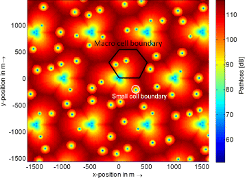

  

  Best path loss map for a HetNet deployment

• The user density and traffic load around the small cell are considered to be uniform, i.e., the load in the micro cell increases linearly with the covered area. This is a reasonable assumption since there is no evidence that the user density is changing at the current cell border.

It needs to be emphasised that those assumptions are only used to do a rough approximation of what cell range expansion might be optimum for the current load situation. However, it is not critical that these conditions are exactly met since the algorithm will dynamically correct the decision based on subsequent network measurements.

Figure 7 shows the lowest path loss map (provides the lowest path loss at each position to any of the radio cells) of a heterogeneous cell deployment according to 3GPP TR36.814 [17] (more specifically scenario 6.2, i.e. macro + outdoor RRH/hotzone with model 1 has been used). This scenario is composed of radio sites with three sectors forming a regular grid of radio cells. In each macro cell area, two small cells are randomly positioned. It can be seen that the macro cells can be well approximated by a hexagon whereas the small cell can be well approximated by a circle. In addition, it needs to be mentioned that the major source of interference in the small cell comes from the macro cell since the path loss of the small cell is increasing fast with larger distance due to the relatively low antenna height and the use of omni-directional antennas for a small cell.

The small cell size can be expanded until either the total small cell load or the load in ABS exceeds the nominal load, i.e. CRE adaptation needs to take into account both load limits. The current total small cell load and the current small cell radius will be defined by L _c and r _c, whereas the nominal cell load and the nominal cell size will be denoted by L _n and r _n. Since the user density is assumed to be homogeneous in the vicinity of the small cell, the following relationship between cell loads can be established:

$$ \frac{\pi \cdot r_{\mathrm{n}}^{2}}{\pi \cdot r_{\mathrm{c}}^{2}} = \frac{L_{\mathrm{n}}}{L_{\mathrm{c}}} \;\;\; \;\;\; \; \; \text{or} \; \; \;\;\; \;\;\; \frac{r_{\mathrm{n}}}{r_{\mathrm{c}}}=\sqrt{\frac{L_{\mathrm{n}}}{L_{\mathrm{c}}}}. $$

((9))

The difference between the currently used cell range expansion C R E _c and the nominal cell range expansion C R E _n can be expressed as the path loss difference between P L _c (pathloss of a user equipment (UE) that is located at a distance r _c from the small cell centre) and P L _n (pathloss of a UE located at a distance r _n from the small cell centre). From Eq. 8, the following relationship can be derived:

$$ \mathrm{{CRE}_{n}-{CRE}_{c}}=\mathrm{{PL}_{n}-{PL}_{c}}=b \cdot \left(\text{log}_{10}\left(r_{\mathrm{n}}/r_{\mathrm{c}}\right)\right). $$

((10))

Inserting Eq. 9 into Eq. 10 yields the following relationship between the load and cell individual offset values:

$$ \mathrm{{CRE}_{n}}=b/2 \cdot \text{log}_{10}(L_{\mathrm{n}}/L_{\mathrm{c}}) - \mathrm{{CRE}_{c}}. $$

((11))

As already discussed earlier, also the load in the ABS subframes needs to be considered when selecting the cell individual offset values. The load in ABS subframes is defined as the load that is created by those UEs that need to be protected from the macro cell interference. In the following, it is assumed that all users that are outside of the normal cell radius r ₀ that is valid for a cell individual offset of 0 need to be protected from macro cell interference since the path loss to the macro cell is lower than the path loss to the small cell. Using the above assumptions, the following equation can be derived:

$$ \frac{\pi \cdot \left(r_{\mathrm{n,ABS}}^{2}-{r_{0}^{2}}\right)}{\pi \cdot \left(r_{\mathrm{c}}^{2}-{r_{0}^{2}}\right)} = \frac{\left(r_{\mathrm{n,ABS}}^{2}-{r_{0}^{2}}\right)}{\left(r_{\mathrm{c}}^{2}-{r_{0}^{2}}\right)}=\frac{L_{\mathrm{n}}}{L_{\mathrm{c,ABS}}}, $$

((12))

where r _n,ABS denotes the nominal cell range due to ABS load and L _c,ABS is equal to the current load in ABS.

The normal cell radius r ₀ can be evaluated from the currently used C R E _c and the current cell size r _c using Eq. 8 as

$$ r_{0}=r_{\mathrm{c}} \cdot 10^{-\mathrm{{CRE}_{c}}/b}. $$

((13))

Finally, we can derive a nominal CRE from ABS load using Eqs. 8, 12 and 13 as

$$\mathrm{{CRE}_{n,ABS}} = \mathrm{{PL}_{n,ABS}-PL}_{0}=b \cdot \text{log}_{10}(r_{\mathrm{n,ABS}}/r_{0}) $$

$$ \mathrm{{CRE}_{n,ABS}} = \frac{b}{2} \cdot \log_{10}\left[\frac{L_{\mathrm{n}} \cdot \left(10^{2 \cdot \mathrm{{CRE}_{c}}/b} - 1\right)}{L_{\mathrm{c,ABS}}} + 1 \right]. $$

((14))

The final maximum CRE to be used is then the minimum of C R E _n and C R E _{n,A B S} . The case of CRE reduction can be handled in a similar way as the CRE expansion.

The dynamic adaptation of the CRE will also affect the load in the almost blank subframes, and therefore, it is also important to dynamically control the ratio between ABS and normal subframes, which will be discussed in the following section. If the dynamic cell range adaptation algorithm and the dynamic ABS adaptation algorithms are both in use, it is important that both work in different time scales. Since the change of the CRE requires signalling to each connected UE, it is recommended to perform the ABS adapation faster than the CRE adaptation to follow the traffic fluctuations as fast as possible.

4.2 Dynamic adaptation of ABS pattern

The dynamic adaptation of the ABS pattern needs to be changed in response to the total load and the load within almost blank subframes for all small cells that are located in the macro coverage. So from a high-level perspective, the number of ABS needs to be increased when the total load of all involved small cells during ABS exceeds the total load in the whole macro area, whereas it can be decreased in the opposite case as shown in Fig. 8.

Fig. 8

Load-based ABS pattern adaptation

This example algorithm has been simulated for the HetNet hotspot scenario 6.2 defined in [17]. So, there are additional users around the small cells (traffic hotspot) and an additional uniform user distribution for the macro cell area. The user ratio between hot spots and uniform user traffic has been selected as 2:1. The basic simulation parameters are summarised in Table 1. Different ABS patterns 0, 1,..., 6 have been defined, where the ratio between ABS and total number of subframes is selected as 0, 12.5,..., 75 %, respectively.

Table 1 Simulation parameters

Users are created dynamically and in the hotspot area that is located around the small cell twice as much users are generated than in the macro area. Figure 9 displays the average ABS pattern for the load-based dynamic ABS adaptation compared to the optimum ABS patterns that have been derived from running the simulation with different static ABS patterns and then showing this pattern that provides the highest 5 % tile UE throughput, 50 % tile UE throughput or cell throughput, respectively. It can be seen that the ABS pattern is increasing with growing CRE since more and more users are served in the small cell CRE area, which requires additional ABS as expected. In addition, it can be observed that the dynamic pattern uses different ABS patterns depending on the load situation, which can be seen from the fact that for a CRE of 2 dB ABS patterns 0 and 1 are selected with roughly equal probability. In general, the dynamic algorithm follows quite closely the optimised patterns derived from static simulations but since it is dynamic, it can also follow the load fluctuations in the network which is not possible with a static ABS pattern. This confirms the benefit of the dynamic algorithm.

Fig. 9

Dynamic ABS adaptation versus static optimisation

Figure 10 shows the dynamics of the number of active users in one macro cell and the underlying four macro cells and the ABS pattern that is selected by the ABS adaptation algorithm. From the time trace, it can be seen that the number of users in the different radio cells is changing dynamically since the users are starting to transmit data and stop transmitting data or do a handover between cells. In the selected scenario, the users are generated dynamically with a Poisson process and then transmitted for approximately 5 s at a constant bit rate and finally leave the system. In addition, they can do handovers due to UE mobility or change of propagation conditions (mainly do to slow fading). All results are valid for the downlink direction since that is the focus of the algorithm. The uplink direction is only indirectly affected since the macro cells are not allowed to send the uplink resource allocations on the physical downlink control channel (PDCCH) during ABS, and the small cell users located in the cell range expansion need to receive the uplink resource allocations during ABS. However, this is not considered further since the downlink is typically much higher loaded than the uplink. It can be seen that the algorithm changes the ABS pattern in response to the downlink traffic load, and there is a tendency to use a higher ABS pattern (providing more ABS) if the ratio of the small cell users to the macro cell users is high since then the load in the small cells especially in the ABS is relatively high. However, there is no strict dependency since the behaviour does also depend on the concrete UE positions and the distribution of the UEs in the small cells.

Fig. 10

Time trace of the number of active users in macro and small cells as well as ABS pattern

This confirms that the described algorithm works well in a distributed environment, where the macro and small cells are served by individual base stations that are interconnected via a normal transport network. It can track load fluctuation in the range of 1 s but it cannot follow extremely fast load fluctuations. A more frequent per subframe selection of normal versus almost blank subframes is possible if the small cells and the macro cells are connected to a single base station as described in [18]. This allows to change between ABS and non-ABS every millisecond whereas the normal adaptation of the ABS pattern is typically every 100 ms–4 s. Other examples of adaptive radio resource management algorithms can be found in the following references:

• Fast dynamic selection of the best radio cell based on load and propagation conditions [19]

• Coordinated muting/scheduling between different radio cells based on interference and load [20]

• Adaptive uplink power control based on intercell interference [21]

5 Self-organising networks

The LTE radio access network (RAN) with its flat network architecture [22] has been designed from the beginning in such a way that it can operate relatively independent from other parts of the network.

Handover of UEs for example is autonomously initiated, prepared, and executed by the LTE base stations (called eNBs) via RAN-internal interfaces (realising 3GPP reference point X2, as shown in Fig. 11) independent of the core network. Only in a final streamlining phase of a handover, the core network is involved to update the routing of control and user data flows.

Fig. 11

Flat LTE RAN network architecture with X2 interfaces between eNBs

Such direct interactions between LTE base stations is also an enabler of distributed SON concepts [23] that replace, complement or enhance traditional centralised network planning and network management techniques with distributed, self-organising and adaptive mechanisms for self-configuration, self-optimisation and self-healing [24].

A key enabler for SON in LTE is a set of 3GPP-standardised functions in the mobile user equipment which allow using these end-user devices as sensors for the network that perform all kinds of measurements and report the results back to the network [2]. Based on input from hundreds or thousands of end-user devices, the SON functions in the network can flexibly adapt the network configuration to changes that may happen on quite different time scales ranging from traffic fluctuations (in the order of seconds or minutes) to changes in the environment (in the order of several hours, days, or even weeks, e.g. when new base stations are set up or when new buildings are constructed that change radio propagation conditions).

In the following, three SON functions in modern 4G networks are briefly characterised.

5.1 Automatic Neighbour Relations

Handover measurements in mobile communications systems, i.e. measurements that are performed by UEs on neighbouring cells while they are connected to a serving cell, are typically related to the so-called Physical Cell ID (PCI) of a neighbour cell. PCIs are tightly coupled to the used radio technology and are relatively easy to detect (which is important so that such measurements do not unnecessarily interrupt the ongoing communication in the serving cell). Such PCIs are however never unique, i.e. the actual global identity of the cell (which is, e.g. needed to organise the handover within the network) cannot be directly derived from a PCI. Therefore, the network needs a mapping table which depending on the geographic location of a cell provides a mapping between measured PCIs and global identifiers of the neighbouring cells. The ANR function in LTE [25] automates the creation and maintenance of such mapping tables and frees the operator from this relatively trivial and cumbersome task. This is achieved by asking UEs to retrieve and report the global cell identity of neighbour cells in periods in which the UE has no data activity in the serving cell and therefore is able to temporarily abandon the serving cell to listen to the broadcasted system information of the neighbour cell (in which the global cell identity is contained). When an eNB has detected a new neighbour, it will not only update its internal mapping tables but will also establish a connection via the X2 interface to the corresponding neighbour eNB which then enables exchange of information for other SON purposes like MRO and MLB. Furthermore, ANR provides the basis for self-configuration and self-optimisation of the PCI allocation to cells, i.e. PCI allocation (for new or already existing cells) can be adapted to the PCIs of the neighbour cells and to the PCIs of the neighbours of the neighbour cells.

In the ideal case, the ANR function even helps to detect neighbour relations which traditional network planning could not find due to restrictions in the underlying modelling of the radio environment and thereby may lead to better handover and SON decisions. Though ANR can be quite fast in reacting to changes in the radio environment, the time scale of changes which is addressed by this functionality is in the order of several hours, days, or even weeks.

An important task of the ANR function is to distinguish between relevant and irrelevant neighbours and to detect if a neighbour relation has become obsolete, e.g. because the corresponding cell was removed or other changes (modified antenna tilt, reduced power, changes in the environment) have made it irrelevant. In dense deployments, we typically see that ANR detects around 40 to 50 (or more) intra-frequency neighbour cells per serving cell. This number is also confirmed by radio simulations, as shown in Fig. 12.

Fig. 12

Simulation results for detected neighbour relations in a real network deployment scenario

If we rank those neighbour relations (NRs) according to the occurrence of handovers and if we then calculate for each NR how many handovers are not covered by the NRs with a lower rank (i.e. with a lower relevance), we get a negative exponential complementary distribution function. As a rule of thumb, we can say that one third of the detected NRs carry 99 % of the handovers and two third of the detected NRs carry around 99.99 % of the handovers, i.e. the remaining third only carries 0.01 % of handovers (which corresponds to 10 HO per day in a cell with 100,000 handovers per day) and the ANR function needs to take this relatively rare occurrence of handovers into account when deciding about set-up or removal of X2 links for such neighbour relations.

5.2 Mobility Robustness Optimisation

While ANR is mainly a SON function for self-configuration, MRO is a function that performs self-optimisation tasks [26]. It optimises the parameters for handover measurements and handover decision algorithms. Again, special functions in the UEs in combination with direct communication between eNBs are used to detect and report issues with handover execution in a distributed fashion. As a reaction to such issues, the eNB may adapt the handover configuration parameters, which were initially provided by the network operator, in a neighbour cell-specific way, i.e. it may decide to apply different thresholds or offsets for handover measurements and decisions depending on the potential target cell of the handover. MRO operates on a time scale in the order of a few minutes to a few hours.

3GPP has specified distributed SON functionality that supports the detection and reporting of the following types of handover issues:

• Too late handovers: Handover command is sent too late to the UE, i.e. the connection in the serving cell dropped due to poor radio conditions before the UE received the handover command.

• Too early handovers: Handover to the target cell is commanded too early, i.e. the UE will not be able to maintain the connection in the target cell because of poor radio conditions while the source cell of the handover would still have been the best choice.

• Handovers to the wrong cell: Handover is commanded to the wrong cell, i.e. the UE will not be able to maintain the connection in the target cell because of poor radio conditions and a third cell would have been the better choice.

• Handover ping-pongs: Even though handovers are carried out successfully, handover algorithms in the involved cells lead to a sequence of several handovers between a small set of cells, e.g. between two cells, in a relatively short period of time.

5.3 Mobility Load Balancing

MLB is a self-optimising SON function [26] that enables distribution of connected UEs (and their corresponding traffic) across cells of the same or of a different radio access technology. Depending on the applied radio resource management (RRM) scheme, different MLB mechanisms may be applied (e.g. a pure overflow mechanism for congestion handling or a load balancing mechanism for optimising quality of experience of individual UEs or specific services) and co-existence with other load balancing mechanisms (like e.g. carrier aggregation and eICIC) needs to be taken into account. MLB addresses a time scale in the order of seconds.

Key enabler for MLB mechanisms is direct communication between network elements to exchange information about resource utilisation and available capacity of various types of resources (e.g. for uplink and for downlink, on the radio interface and in the transport backbone). Within LTE, this direct information exchange is carried out via X2 and may operate on a time scale of a few seconds. Towards other radio access technologies, communication is carried via the core network to the controlling network elements of the other radio access technology (e.g. towards UMTS radio network controllers) using the so-called RAN Information Management (RIM) protocol.

6 Conclusions

Different adaptive techniques have been presented for different layers of a cellular wireless network based on the LTE-Advanced standard. These techniques are working on top of each other and have to cover a large time scale in order to react appropriately to the different environmental changes, e.g., in the radio channel and in the user traffic. The interdependency between the different adaptive algorithms has to be taken into consideration carefully in order to achieve an optimal capacity of the wireless network. A typical examples is the interaction between the SON functions, MRO and MLB, respectively, and the dynamic cell range adaptation used in heterogeneous networks. The distribution of traffic between a macro cell and several micro cells in heterogeneous networks taking into account the overhead of the signalling for the feedback information is another example. The wide range of capabilities for the mobile and base stations in a LTE-A-based cellular wireless network adds an additional complexity for these adaptive algorithms.

The future 5G standard for cellular wireless networks, which will be based on larger bandwidth, much higher number of antennas and more sophisticated cell deployments, will require most likely even more sophisticated adaptive techniques.

References

CE Shannon, W Weaver, The Mathematical Theory of Communication (University of Illinois Press, Illinois, 1949).
S Sesia, I Toufik, M Baker, LTE —the UMTS Long Term Evolution (John Wiley & Sons, Chichester, West Sussex, UK, 2011).
M Bossert, B Haetty, P Klund, in ITG-Fachbericht 124. Propagation aspects on railway environment in the GSM frequency range (Informationstechnische GesellschaftFrankfurt, Germany, 1993), pp. 319–330.
G Fettweis, M Lohning, D Petrovic, M Windisch, P Zillmann, W Rave, in IEEE 16th International Symposium on Personal, Indoor and Mobile Radio Communications, 2005. PIMRC. Dirty, RF: a new paradigm (IEEEBerlin, Germany, 2005).
PB Kenington, High-Linearity RF Amplifier Design (Artech House, London, 2000).
E Aschbacher, Digital pre-distortion of microwave power amplifiers. PhD thesis. Technische Universität Wien, Fakultät für Elektrotechnik und Informationstechnik (2005).
M Schetzen, The Volterra and Wiener Theories of Nonlinear Systems (John Wiley, New York, 1980).
3GPP TS 45.005: Technical specification group GSM/EDGE radio access network; radio transmission and reception (Release 12, March 2015). http://www.3gpp.org.
A Splett, H-J Dreßler, A Fuchs, R Hofmann, B Jelonnek, H Kling, E Koenig, A Schultheiß, in IEEE 2001 Custom Integrated Circuits Conference, CICC. Solutions for highly integrated future generation software radio basestation transceivers (IEEESan Diego, USA, 2001).
TH Lee, The Design of CMOS Radio-Frequency Integrated Circuits (Cambridge University Press, Cambridge, 2004).
H Holma, A Toskala, LTE for UMTS Evolution to LTE-Advanced (John Wiley & Sons, Chichester, West Sussex, UK, 2011).
E Dahlman, S Parkvall, J Sköld, 4G LTE/LTE-Advanced for Mobile Broadband (Academic Press, Oxford, UK, 2011).
3GPP TS 36.213: Technical specification group radio access network; Evolved Universal Terrestrial Radio Access (E-UTRA); physical layer procedures (Release 12, June 2015). http://www.3gpp.org.
3GPP TR 36.897: Technical specification group radio access network; study on elevation beamforming/full-dimension (FD) MIMO for LTE (Release 13, July 2015). http://www.3gpp.org.
EU Project METIS: Mobile and wireless communications enablers for the twenty-twenty information society. https://www.metis2020.com.
M Nohrborg, Self-organizing networks (SON). http://www.3gpp.org/technologies/keywords-acronyms/105-son.
3GPP TR 36.814: Technical specification group radio access network; Evolved Universal Terrestrial Radio Access (E-UTRA); further advancements for E-UTRA physical layer aspects (Release 9, March 2010). http://www.3gpp.org.
B Soret, K Pedersen, T Kolding, H Kroener, I Maniatis, in GLOBECOM. Fast muting adaptation for LTE-a HetNets with remote radio heads (IEEEAtlanta, USA, 2013), pp. 3790–3795.
R Agrawal, A Bedekar, R Gupta, S Kalyanasundaram, H Kroener, B Natarajan, in WCNC. Dynamic point selection for LTE-advanced: algorithms and performance (IEEEIstanbul, Turkey, 2014), pp. 1392–1397.
R Agrawal, A Bedekar, S Kalyanasundaram, N Arulselvan, T Kolding, H Kroener, in Spring. Centralized and decentralized coordinated scheduling with muting (IEEESeoul, Korea, 2014), pp. 1–5.
M Sen, S Kalyanasundaram, R Agrawal, H Kroener, in VTC Fall. Performance analysis of interference penalty algorithms for LTE uplink in heterogeneous networks (IEEEVancouver, Canada, 2014), pp. 1–5.
3GPP TS 36.300: Technical specification group radio access network; Evolved Universal Terrestrial Radio Access (E-UTRA) and Evolved Universal Terrestrial Radio Access Network (E-UTRAN); overall description; Stage 2 (Release 10, January 2015). http://www.3gpp.org.
3GPP TS 32.500: Technical specification group services and system aspects; telecommunication management; self-organizing networks (SON); concepts and requirements (Release 10, October 2010). http://www.3gpp.org.
S Hämäläinen, H Sanneck, C Sartori, LTE Self-Organizing Networks (SON) (John Wiley & Sons, Chichester, West Sussex, UK, 2012).
3GPP TS 32.511: Technical specification group services and system aspects; telecommunication management; automatic neighbour relation (ANR) management; concepts and requirements (Release 10, March 2011). http://www.3gpp.org.
3GPP TR 36.902: Technical specification group radio access network; Evolved Universal Terrestrial Radio Access Network (E-UTRAN); self-configuring and self-optimizing network (SON) use cases and solutions (Release 9, April 2011). http://www.3gpp.org.
Acknowledgements
The authors would like to thank their colleagues from Nokia Networks for valuable comments and suggestions and for preparing the simulation results.
Author information
Authors and Affiliations
Corresponding author
Additional information
Competing interests
The authors declare that they have no competing interests.
Rights and permissions
Open Access This article is distributed under the terms of the Creative Commons Attribution 4.0 International License (http://creativecommons.org/licenses/by/4.0/), which permits unrestricted use, distribution, and reproduction in any medium, provided you give appropriate credit to the original author(s) and the source, provide a link to the Creative Commons license, and indicate if changes were made.
About this article
Cite this article
Hätty, B., Dreßler, HJ., Kröner, H. et al. Adaptive techniques in advanced 4G cellular wireless networks. EURASIP J. Adv. Signal Process. 2016, 19 (2016). https://doi.org/10.1186/s13634-016-0310-x
Received:
Accepted:
Published:
DOI: https://doi.org/10.1186/s13634-016-0310-x