- Research
- Open access
- Published:
Singular spectrum-based matrix completion for time series recovery and prediction
EURASIP Journal on Advances in Signal Processing volume 2016, Article number: 66 (2016)
Abstract
Big data, characterized by huge volumes of continuously varying streams of information, present formidable challenges in terms of acquisition, processing, and transmission, especially when one considers novel technology platforms such as the Internet-of-Things and Wireless Sensor Networks. Either by design or by physical limitations, a large number of measurements never reach the central processing stations, making the task of data analytics even more problematic. In this work, we propose Singular Spectrum Matrix Completion (SS-MC), a novel approach for the simultaneous recovery of missing data and the prediction of future behavior in the absence of complete measurement sets. The goal is achieved via the solution of an efficient minimization problem which exploits the low rank representation of the associated trajectory matrices when expressed in terms of appropriately designed dictionaries obtained by leveraging the theory of Singular Spectrum Analysis. Experimental results in real datasets demonstrate that the proposed scheme is well suited for the recovery and prediction of multiple time series, achieving lower estimation error compared to state-of-the-art schemes.
1 Introduction
The dynamic nature of Big Data, a feature termed velocity, is a critical aspect of massive data streams from a signal processing viewpoint [1]. Due to the high velocity of the input streams, measurements may be missing with a high probability. This phenomenon can be attributed to three factors, namely: (a) intentionally collecting a subset of the measurements for efficiency purposes; (b) unintentional subsampling due to desynchronization; and (c) missing measurements due to communications errors including packet drops, outages, and congestion. To elaborate on these factors, we consider data streams associated with the Internet-of-Things (IoT) paradigm and we focus on Wireless Sensor Networks (WSNs) since WSNs can serve as an enabling platform for IoT applications [2, 3]. In the context of IoT/WSNs, one source of missing measurements is attributed to intentional subsampling, a scenario where the designer/operator reduces the sampling rate of the sensing infrastructure in order to increase the lifetime of the network. The relationship between sampling rate and lifetime is governed by the limited energy availability that typically characterizes WSNs. While efficient compression and aggregation schemes can be employed to reduce power consumption, reducing the number of measurements is the most efficient approach to achieve this goal [4].
Even when a specific sampling rate is selected, desynchronization between nodes inevitably leads to a reduction of the network-wide sampling rate, since nodes that were supposed to sample at the same time instance end up acquiring measurements at different instances [5]. This issue is also closely related to the quantization of the sampling time, as measurements that were collected in succession can be mapped to different sampling instances, introducing missing measurements for particular time slots. In addition to energy consumption and desynchronization, missing measurements can also be attributed to network outages and packet losses, which are frequent in WSNs deployed in harsh and cluttered environments, causing a large number of packets to fail in reaching their destination.
In this work, we investigate a novel paradigm in distributed data acquisition and centralized reconstruction and forecasting. The proposed sampling, reconstruction, and prediction scheme assumes that only a small number of randomly selected nodes acquire measurements during each sampling instance, while nodes that are not in the sampling group enter a low-power state. Because of the sampling scheme, in addition to missing data due to packet losses, the base station only observes a subset of the entire collection of measurements. To address this issue, we propose the so-called Singular Spectrum Matrix Completion (SS-MC) scheme, a formal approach for the recovery of missing values and the forecasting of future ones from a single or multiple time series measurements. The proposed SS-MC scheme builds upon the recently proposed framework of Matrix Completion (MC) [6, 7] for the recovery of low-rank matrices from a minimal set of measurements by extending the low-rank matrix recovery framework to the estimation of missing measurements from appropriately generated trajectory matrices and combines it with the Singular Spectrum Analysis framework for exploiting the information encoded in training data. Figure 1 presents a visual overview of the proposed reconstruction scheme, where incomplete trajectory matrices are recovered, providing accurate estimations of past and future measurements. In short, the key novelties of this work include the following:
-
A novel efficient paradigm for estimating missing measurements which extents the recently developed framework of low-rank matrix recovery by exploiting inherent correlations without the need for explicit models.
Fig. 1 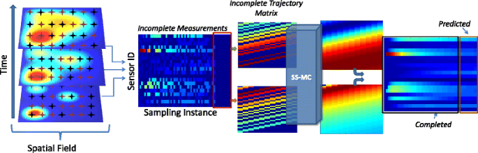
Overview of the proposed sampling, recovery, and prediction scheme. On the left, the three images correspond to the spatial field at three different time instances, where the star symbols indicate the sensing nodes. During each sampling instance, red stars indicate sampling sensors while black stars indicate non-sampling sensors. The figure in the center depicts the incomplete measurement matrix where rows correspond to measurements from a specific sensor and columns to different sampling instances. The red square over the right part of the matrix highlights that in addition to missing value estimation, our system can generate a number of instances (columns) corresponding to future predictions. Individual sensor measurements are transformed to trajectory matrices that are introduced to the proposed SS-MC framework. The SS-MC algorithm produces completed trajectory matrices that can be joined to generate a fully completed (past and future) measurement matrix
-
The proposed SS-MC scheme is an integrated approach for accurately predicting future values even when only a limited number of past measurements is available. This is radical departure from traditional time series forecasting schemes which assume the full availability of historical data.
-
The proposed scheme can naturally handle a single or multiple time series sources extending traditional estimation approaches that operate strictly on either single or multi-source data.
-
The performance of the proposed method against state-of-the-art techniques is evaluated on real data acquired by a distributed sensor network, which serves as an illustrative example of a Big Data application.

The rest of the paper is organized as follows: Section 2 presents an overview of state-of-the-art methods for energy-efficient data collection. Sections 3 and 4 provide the description of the two theoretical models we consider in this work, namely time series modeling via Singular Spectrum Analysis and missing measurement estimation via the Matrix Completion framework. Section 5 introduces SS-MC, our proposed recovery and prediction method, including the mathematical formulation as well as an efficient optimization approach based on Augmented Lagrange Multipliers. The performance of the proposed scheme is experimentally validated against state-of-the-art methods in Section 6 and the paper concludes in Section 7.
2 Related work
Designing efficient techniques for minimizing the cost of continuous data collection by exploiting data correlations has been extensively studied from multiple aspects and different perspectives in the context of WSNs [8]. Jindal and Psounis [8] presented a method for inferring the spatial correlation of WSN data and for generating synthetic data using a statistical tool called variagriam. Estimating the sampling field at a given location, based on the available sensor data at other additional locations is a common approach for energy efficient sampling. Data imputation and interpolation techniques, such as Nearest Neighbors Imputation and Kriging, are two very efficient schemes for estimating unavailable data [9]. While in interpolation, one seeks the value of the field in a location where no sensors are present, imputation approaches try to estimate the value at the sensor location at a time instance where sampling did not take place. Kriging relies on the semi-variogram, a statistical tool developed by geo-statisticians [10] in order to estimate the value of a field at a specific location, given prior knowledge about the inherent correlations of data from neighboring nodes. In k-Nearest Neighbors, this objective is reached by using a weighted nearest neighbor interpolation, where the weight corresponding to each sample is based on statistical information indicating the degree of spatial dependence in the field [11].
Another line of work for data imputation exploits probabilistic models for estimating the missing entries. In [12], an Expectation Maximization (EM) algorithm is presented which estimates the parameters of the probability distribution of the data by iteratively maximizing the likelihood of the available data as a function of these parameters. In order to increase the robustness of the process, the authors proposed the regularized EM (RegEM) where a regularization term is added during the inversion of the correlation matrix in order to increase the robustness of the algorithm when more variables are present than data records. RegEM is currently one of the state-of-the-art data imputation techniques, and its performance is compared against the proposed and other schemes in the experimental section.
Data compression has also been extensively explored in the context of energy-efficient data collection in WSNs, based on the premise that data processing is less demanding in terms of energy consumption compared to transmission; hence, energy reduction can be achieved. For example, the recently proposed framework of Compressed Sensing (CS), a state-of-the-art signal sampling and compression scheme, was investigated for WSN data acquisition and aggregation [13, 14] exploiting the sparsity of the sampled data when expressed in an appropriate basis [15]. Distributed compression schemes such as Distributed Source Coding [16] have also been proposed for compressing WSN measurements in densely deployed networks, since utilizing side information from neighboring nodes can dramatically reduce communication cost. The sparse characteristics of correlated datasets have also been recently considered for transmission of EEG signals [17, 18]. Although sparsity and CS-based methods can have a dramatic reduction in transmission power, typically in these scenarios, the signals are first fully sampled and then compressed.
While the CS framework requires a particular form of sampling (incoherent sampling), the related paradigm of low-rank matrix recovery (MC) assumes a random sampling of the matrix entries. Due to the intuitive sampling, the MC framework has been considered for a variety of signal recovery problems including collaborative spectrum sensing [19], sensor localization [20, 21], and image reconstruction problems [22, 23] among others. MC has been recently explored as a sampling scheme for WSNs [24–27]. In [24], the authors investigated the scenario where sensors lie on a uniform rectangular grid and random sub-sampling is taking place by each sensor. Our work bares some similarities with this line of work; however, we do not pose specific deployment constraints and we allow the sensors to occupy any location in the sensed region. Furthermore, our work differs significantly in the exploitation of prior knowledge in the form of a dictionary, which is utilized during the reconstruction stage. The utilization of the singular spectrum dictionary allows for the incorporation of prior knowledge regarding the data generation process which can significantly improve the reconstruction performance [25]. Furthermore, the proposed scheme is able to predict future measurements in addition to estimating missing past ones.
Low-rank recovery was also recently considered in [28] where the authors employ MC for the recovery of undersampled correlated EEG signals. Our work in this paper investigates different extensions of MC-based recovery by considering trajectory matrices and singular spectrum dictionaries. We develop a generative model where the sampled data can be jointly represented as a low-rank linear combination of dictionary elements, spanning the subspace where data is lying. A similar situation was recently explored, leading to the low rank representations (LRR) framework [29] where the objective is to identify a low rank matrix which can accurately represent the source data. LRR has been considered for subspace clustering problems [30]; however, only fully populated matrices were considered.
In the context of Big Data, matrix and tensor data recovery via an online rank minimization process [31] was recently proposed for scalable imputation of missing data. This was achieved by low-dimensional subspace tracking through the minimization of a weighted least squares regression, regularized with a nuclear norm. While this work bares resemblance to our work, our generative model does not require a fixed bilinear factorization due to a pre-specified rank, while it exploits the subspace identified by the SSA for simultaneous missing past measurement imputation and future predictions.
3 Analysis of time series data
Singular Spectrum Analysis (SSA) is a model-free method for time series analysis and forecasting which has been widely exploited in the analysis of environmental, economical, and computer network data [32, 33]. The basic assumption underlying SSA is that one can approximate a time series \(\mathbb {M}_{i}\) of length K from L lagged samples, by considering the spectral analysis of specialized matrices, called trajectory matrices. Embedding at sampling instance T, the first step of SSA, involves the process of generating a trajectory matrix \({\mathbf M}_{i}=\{\mathbf {m}_{i,t} \vert t=T-L:T\} \in \mathbb {R}^{K \times L}\) of lag L measurement vectors, where each vector \(\phantom {\dot {i}\!}\mathbf {m}_{i,t'}=\{m_{i,t'} \vert t'=t-K:t \}\) encodes the measurements corresponding to a sampling window of length K for sensor i. The length K of the time window and the lag L are two critical parameters encoding important aspects of the underlying data.
In SSA, once the trajectory matrix of the time series has been generated, the subsequent step involves the spectral analysis of the lag-covariance matrix. Formally, given the matrix M i , the lag-covariance matrix defined as \({\mathbf C}_{i}={\mathbf M}_{i}{\mathbf M}_{i}^{T}\) can be used for extracting the eigenvectors of C which define an L-dimensional subspace where the time series \(\mathbb {M}_{i}\) resides, while the associated eigenvalues encode the variance along the direction of the associated eigenvector. Alternatively, one can apply the SVD decomposition to the original trajectory matrix M i in which case the outputs are two matrices containing the right and left singular vectors U and V and a diagonal matrix Σ containing the singular values. Given the SVD decomposition, the trajectory matrix M i can be expressed as the sum of rank-1 matrices given by \({\mathbf M}_{j}=\sum _{j} \sqrt {\lambda _{j}}\mathbf {u}_{j} \mathbf {v}_{j}^{T}\), where each collection (λ j ,u j ,v j ) is called eigentriple.
Given the eigenvectors extracted via the SSA, one can project and reconstruct the time series or perform prediction by employing two steps, eigentriple grouping and diagonal averaging. Eigentriple grouping aims at arranging the eigentripes in sets in order to separate additive components that are exactly or approximate separable, facilitating the analysis of the eigenvectors. Diagonal averaging aims at translating the recovered trajectory matrix into a time series according to
where m ∗[i,j]=m[i,j] for L<K and m ∗[i,j]=m[j,i] otherwise.
It is worth noting that SSA has also been considered in situations when a number of measurements are missing. A straightforward approach, also employed here, is to estimate the eigenvectors and eigenvalues using only the available measurements during the lag-covariance matrix generation [34]. SSA has also been considered when missing measurements are present [35, 36]; however, the proposed methods differ from our work in that we exploit prior knowledge in the form of a dictionary. Furthermore, the proposed scheme is able to perform missing value estimation, either past or future, while there is no constraint associated with the structure of the missing measurements.
In addition to the analysis of time series, SSA can also be used as a forecasting mechanism. In recurrent forecasting SSA, the time series of known measurements and unknown components is transformed to its Hankel form and the linear recurrent relation coefficients are utilized for forecasting the future values. While typical SSA considers the trajectory matrices associated with a single time series, the Multivariate Singular Spectrum Analysis (MSSA) method has been proposed for handling multiple time series [37–39]. In this work, we consider a simple extension of SSA where instead of analyzing a single trajectory matrix, we consider a compound trajectory matrix generated by the concatenation of S individual matrices, i.e., \(\mathbf {M}=\;[\mathbf {M}_{1}, \mathbf {M}_{2}, \ldots, \mathbf {M}_{S}] \in \mathbb {R}^{S(K \times L)}\). Introducing multiple sources of data can have a dramatic impact in performance as will be shown in the experimental results, with at most linear increase in computational complexity.
4 Low-rank matrix completion
The low-rank approximation of a given matrix is a frequent problem in data analysis [40]. The rank of the matrix indicates the number of linearly independent columns (or rows), and thus it is a indicator of the degree of linear correlation that exists within the data. There are multiple reasons that justify the need for such an analysis. For example, prior knowledge regarding the linear correlation of the data may suggest that the requested matrix is low rank. In other situations, noise in the data artificially increases the rank of the matrix, so reducing the rank effectively amounts to a denoising process. Assuming without loss of generality that S=1, given a noisy (K×L) matrix M, the objective of low-rank approximation is to identify a matrix X such that:
where ε is the approximation error, related to the noise power. By utilizing the SVD decomposition M=U S V T, a low-rank approximation matrix X can be found by \({\mathbf {X}}=\mathbf {U} \mathcal {T}(\mathbf {S}) \mathbf {V}^{T}\), where \(\mathcal {D}_{\tau }(\mathbf {S})=diag([\sigma _{i}(\mathbf {S})-\tau ]_{+})\) is a thresholding operator that selects only the elements with values greater than τ from the diagonal matrix S and sets the rest to zero. The effect of this process is that only a small number of singular values are kept for the low-rank approximation X of M.
The rank of the matrix is a key property in the recently proposed framework of Matrix Completion (MC) where one tries to estimate the (K×L) entries of the matrix M from a smaller number of q entries, where q≪(K×L). According to MC, such a recovery is possible provided the matrix is characterized by a small rank (compared to its dimensions) and enough randomly selected entries of the matrix are acquired [6, 41]. More specifically, one can recover an accurate approximation X of the matrix M from a small number of entries by solving the minimization problem:
where \(\mathcal {P}_{\Omega }\) is a random sampling operator which records only a small number of entries from the matrix M, i.e.,
where Ω is the sampling set. In the context of WSN for example, the set Ω specifies the collection of sensors that are active at each specific sampling instance. In general, to solve the MC problem, the sampling operator \(\mathcal {P}\) must satisfy the modified restricted isometry property, which is the case when uniform random sparse sampling is employed in both rows and columns of matrix M [42]. The incoherence of sampling introduced by \(\mathcal {P}\) with respect to M guarantees that recovery is possible from a limited number of measurements.
Although solving the above problem will generate a low-rank matrix consistent with the observations, rank minimization is an NP-hard problem. Fortunately, a relaxation of the above problem was shown to produce very accurate approximations, by replacing the rank constraint by the tractable nuclear norm, which represents the convex envelope of the rank [6]. The minimization in Eq. (4) can then be reformulated as:
where the nuclear norm is defined as \(\|{\mathbf X}\|_{*}=\sum \|\sigma _{i}\|_{1}\), i.e., the sum of absolute values of the singular values. Candès and Tao showed that under certain conditions the nuclear norm minimization in Eq. (5) can estimate the same matrix as the rank minimization in Eq. (3) with high probability provided q≥C K 6/5 r l o g(K) randomly selected entries of the rank r matrix are acquired [7] (assuming K≥L).
To solve the nuclear norm minimization problem, various approaches have been proposed including Singular Value Thresholding [43] and the Augmented Lagrange Multipliers [44], among others. We review the technique based on the ALM due to its exceptional performance in terms of both processing complexity and reconstruction accuracy and since it is used as a basis for the extended scheme we discuss next.
To express the MC problem in Eq. (5) in the ALM form, we reformulate it as:
The additional variable E is introduced in order to encode the unknown values in the trajectory matrix M, by restricting the estimation error on the recorded values only. The optimization encoded in Eq. (6) can be expressed in an augmented Lagrangian form by defining the Lagrangian function:
where Y is the Lagrange multiplier matrix associated to the first equality constraint and μ is the penalty parameter. Minimization of the problem in Eq. (7) involves an iterative process, where a sequential minimization over all variables, i.e., X,E, and Y, takes place at each iteration. This method of iteratively minimizing over each variable is refereed to as the Alternating Directions Method of Multipliers (ADMM) [45, 46].
One of the key characteristics of MC is the minimal conditions that are imposed for successful recovery, namely the incoherence of sampling and the low rank of the recovered matrix. While a minimal set of requirements is beneficial in situations where limited prior information is available, when such information exists introducing additional constraints can lead to a significantly better recovery. In this section, we exploit the temporal dynamic that time series exhibit in order to enhance typical MC with an additional dictionary which encodes past behavior in a proposed SS-MC framework.
5 The SS-MC algorithm
We consider the truncated trajectory matrices M formed by concatenating the individual trajectory matrices according to the MSSA approach. The objective of this work is to consider a generative model that produces the time series Hankel matrices M according to the factorization M = D L where M may correspond to a single or multiple sources. In both cases, our key assumption is that given a full rank dictionary matrix D obtained through training data, the coefficient matrix L is approximately low rank, i.e., the number of significant singular vectors is much smaller than the ambient dimensions of the matrix.
To apply the low-rank representation scheme on matrices with missing data, the introduction of the random sub-sampling operator is necessary. Our proposed sampling scheme is a combination of MC and reduced rank multivariate linear regression and it seeks a low-rank presentation coefficient matrix L from a small number of measurements \(\mathcal {P}_{\Omega }(\mathbf {M})\). Based on this generative model, our proposed Singular Spectrum Matrix Completion (SS-MC) formulation is given by:
where D is a dictionary of elementary atoms that span a low-rank data-induced subspace. Figure 2 presents an example of a real trajectory matrix (left), the representations coefficients L (center), and the singular value distribution of the coefficients (right).

Example of the generative process of a real trajectory matrix from the Intel-Berkeley dataset. The matrix on the left is the Hankel matrix generated by a sensor for a given set of window and lag values. By utilizing the SSA-based dictionary, the mapping of the Hankel matrix results in an extremely low rank representation matrix shown in the middle, where a small number of singular values capture most of the signal energy, as shown in the right figure
5.1 Efficient optimization
Similarly to MC optimization, the problem in Eq. (8) is NP-hard due to the rank in the objective function and thus it cannot be solved efficiently for reasonably sized data. A remedy to this problem is to replace the rank constraint with the nuclear norm constraint, thus solving:
A key novelty of our work is that in addition to the low rank of the matrix, during the recovery, we employ a dictionary for modeling the generative process that produces the sensed data, as it can be seen in Eq. (9).
The problem in Eq. (9) can be transformed to a semidefinite programming problem and solved using interior point methods [47, 48]. However, utilizing such off-the-shelf solvers introduces a very high algorithmic complexity which renders them impractical, even for moderately sized scenarios. Motivated by the requirements for a data collection mechanism that is both accurate and efficient, we reformulate the SS-MC problem in an Augmented Lagrangian form. By utilizing the ALM formulation for SS-MC, we can achieve efficient recovery, tailored to the specific properties of the problem. Introducing the intermediate dummy variables Z and E, Eq. (9) can be written as:
where L , Z, and E are the minimization variables. The extra variable Z is introduced in order to decouple the minimization variables by separating the L variable in the objective function with the Z variable in the first constraint. Similar to the ALM formulation for MC in Eq. (7), E is introduced in order to account for the missing entries in M. More specifically, the constraint on the error matrix E is applied only on the available data via the sampling operator \(\mathcal {P}\). The ALM form of Eq. (10) is an unconstrained minimization given by:
where Y 1 and Y 2 are Lagrange multiplier matrices. The solution can be found by iteratively minimizing Eq. (11) with respect to each of the variables via an ADMM approach. Formally, the minimization problem with respect to L is given by:
The sub-problem in Eq. (12) is a nuclear norm minimization problem and can be solved very efficiently by the Singular Value Thresholding operator [43]. The minimization with respect to Z is given by:
Calculating the gradient of the expression in Eq. (13), we obtain:
which after setting it equal to zero provides the update equation for Eq. (14) given by:
Furthermore, the augmented Lagrangian in Eq. (11) has to be minimized with respect to E, i.e.,
which provides the update equation for Eq. (16) that is given by:
where the notation \(\mathcal {P}_{\not {\Omega }}\) is used to restrict the error estimation only on the measurements that do not belong to the sampling set. Last, we perform updates on the two Lagrange multipliers Y 1 and Y 2. The steps at each iteration of the optimization are shown in Algorithm 1.

Due to its numerous applications, the ADMM method has been extensively studied in the literature for the case of two variables [45, 46] where it has been shown that under mild conditions regarding the convexity of the cost functions, the two-variables ADMM converges at a rate \(\mathcal {O}(1/r)\) [49]. Although extending the convergence properties to a larger number of variables has not been shown in general, recently the convergence properties of ADMM for a sum of two or more non-smooth convex separable functions subject to linear constraints were examined [50].
The proposed minimization scheme in Eq. (11) satisfies a large number of the constraints suggested in [50] such as the convexity of each sub-problem, the strict convexity and continuous differentiability of the nuclear norm, the full rank of the dictionary, and the size of the step for the dual update α, while empirical evidence suggests that the closed form solution of each sub-problem allows the SS-MC algorithm to converge to an accurate solution in a small number of iterations.
5.2 Singular spectrum dictionary
In this work, we investigate the utilization of prior knowledge for the efficient reconstruction of severely under-sampled time series data. To model the data, we follow a generative scheme where the full collection of acquired measurements is encoded in the trajectory matrix \(\mathbf {M} \in \mathbb {R}^{K \times L}\). M is assumed to be generated from a combination of a dictionary \(\mathbf {D} \in \mathbb {R}^{K \times K}\) and a coefficient matrix \(\mathbf {L} \in \mathbb {R}^{K \times L}\) according to M = D L, where we assume that K≤L. This particular factorization is related to SVD by M = D L = U ( S V T) where the orthonormal matrix D = U is a basis for the subspace associated with the column space of M, while L = S V T is a low-rank representation matrix encoding the projection of the trajectory matrix onto this subspace.
This particular choice of dictionary D implies a specific relationship between the spectral characteristics of the trajectory matrix M and the low-rank representation matrix L. To understand this relationship, we consider the spectral decomposition of each individual matrix in the form D=U G 1 R −1 and L=R G 2 V ∗ The matrices U , R and V are unitary while G 1 and G 2 are diagonal matrices containing the singular values of the D and L, respectively. The particular factorization permits us to utilize the product SVD [51, 52] and expresses the singular value decomposition of the product according to the expression D L=U(G 1 G 2)V ∗, where the singular values of the matrix product are given by the product of the singular values of the corresponding matrices.
In this work, we consider orthogonal dictionaries, as opposed to overcomplete ones. Orthogonality of the dictionary guarantees that the vectors encoded in the dictionary span the low-dimensional subspace and therefore the representation of the measurements is possible. Furthermore, an orthonormal dictionary, such as the one considered in this work, is characterized by G 1=I, leaving G 2 responsible for the representation. We target exactly G 2 in our problem formulation by seeking a low-rank representation matrix L.
In our experimental results, we consider sets of training data associated with fully sampled time series from the first days of each experiment for generating the dictionaries. The subspace identified by the fully sampled data is used for the subsequent recovery of past measurements and prediction of future ones. Alternatively, the dictionary could be updated during the course of the SS-MC application via an incremental subspace learning method [53, 54]. We opted out from an incremental subspace learning since although it can potentially lead to better estimation, it is also associated with increased computational load and the higher probability of estimation drift and lower performance.
5.3 Networking aspects of SS-MC
In the context of IoT applications utilizing WSN infrastructures, communication can take place among nodes, but most typically between the nodes and the base station where data analytics are extracted. This communication can be supported (a) by a direct wireless link between the nodes and the sink/base station; (b) via appropriate paths that allow multi-hop communications; or (c) via more powerful cluster heads what forward the measurements to the base station.
For the multi-hop scheme, equal weight of each sample (democratic sampling) implies that no complicated processing needs to take place by the resource limited forwarding nodes. Furthermore, for high-performance WSNs, where point-to-point communication between nodes is available and processing capabilities are sufficient, nodes could perform reconstruction of a local neighborhood thus offering advantages similar to other distributed estimation schemes [55].
From a practical point-of-view, we argue that recovery and prediction of measurements from low sampling rates offer numerous advantages. First, it saves energy by reducing the number of samples that have to be acquired, processed, and communicated thus increasing the lifetime of the network. The proposed sampling scheme also reduces the frequency of sensor re-calibrations for sensors that perform complex signal acquisition, including chemical and biological sampling. As a result, higher quality measurements and therefore more reliable estimation of the field samples can be achieved. Furthermore, the method increases robustness to communication errors by estimating measurements included in lost or dropped packets, without the need for retransmission. Last, our scheme does not require explicit knowledge of node locations for the estimation of the missing measurements, since the incomplete measurement matrices and the corresponding trajectory matrices are indexed by the sensor id, thus allowing greater flexibility during deployment.
6 Experimental results
To evaluate the performance of the proposed low-rank reconstruction and prediction scheme, we consider real data from the Intel Berkeley Research Lab dataset1 [56] and the SensorScope Grand St-Bernard dataset2 [57]. The former dataset contains the recordings of 54 multimodal sensors located in an indoor environment over a 1-month period, while the latter contains multimodal measurements from 23 stations deployed at the Grand-St-Bernard pass between Switzerland and Italy.
In both cases, we analyze temperature measurements as an exemplary modality, while we exclude failed sensors from the recovery process. Unless stated otherwise, in all cases, we fix the SSA parameters, K=50 and L=100, and we train using a single day’s worth of data while testing on the five consecutive ones. The threshold τ for the singular value thresholding operator is set to preserve 90 % of the signals’ energy, while the parameter μ was set to 0.01 through a validation process, although the specific value had a minimal impact in performance.
To evaluate the performance, we consider three state-of-the-art methods and we compare them to the proposed SS-MC. More specifically, we evaluate the performance of the ADMM version of MC [44], the Knn-imputation [58], and the RegEM [12]. The reconstruction error is measured by the normalized mean squared error between the true M and the estimated X trajectory matrices given by \(\frac {\sum \|\mathbf {M-X}\|^{2}}{\sum \|\mathbf {M}\|^{2}}\).
6.1 Recovery with respect to measurement availability
The objective of this subsection is to present the recovery capabilities of the proposed SS-MC and state-of-the-art methods with respect to the availability of measurements, i.e., the sampling rate.
The two plots shown in Fig. 3 present the reconstruction error for the Intel-Berkeley data at 20 % (top) and 50 % (bottom) sampling rates, averaged over all sensing nodes. Naturally, one can see that increasing the sampling rate has a positive effect on all methods. Nevertheless, we also observe that not all sampling instances are equally difficult to estimate and that the reconstruction error exhibits a periodic trend across sampling instances. These variations are attributed to the significant changes in the environmental conditions due to the transition from nighttime to daytime.

Reconstruction error at 20 % (top) and 50 % (bottom) sampling rates for the Intel-Berkeley dataset
Comparing the four methods, we observe that under all measurement availability scenarios, the proposed SS-MC scheme typically achieves the lowest reconstruction error and exhibits the most stable performance. The performance of SS-MC is closely followed, especially in low sampling rates, by RegEM which also exhibits a very stable performance, while on the other hand, MC and Knn-impute are more sensitive to the sampling instance, exhibiting a more erratic behavior.
To further illuminate the behavior of each method, we consider a large set of sampling instances and present the averaged recovery performance as a function of the sampling rate in Fig. 4 for Intel-Berkeley (top) and SensorScope (bottom) data. Regarding the performance on the Intel-Berkeley dataset, we observe that the proposed SS-MC and RegEM achieve comparable performance, much better than typical MC and Knn-impute. An interesting observation is that while SS-MC, RegEM, and Knn-impute all exhibit a monotonic reduction in reconstruction error at higher sampling rates, MC reaches a performance plateau around a 25 % sampling rate. This phenomenon is attributed to the rank constrains of MC leading to a low rank estimation which causes an incorrect estimation of missing measurements.

Average reconstruction error for the Intel-Berkeley (top) and the SensorScope (bottom) platforms
Regarding the performance on the SensorScope data, one can observe that in this case RegEM achieves a significantly better performance compared to the other methods, followed by MC at low sampling rates and SS-MC at large ones. Similar to the behavior observed for the Intel-Berkeley data, MC again reaches a performance plateau while the other methods achieve a monotonically reducing reconstruction error. Note that although RegEM achieves the lowest reconstruction error, it is also the most computationally demanding of the four methods.
6.2 Recovery from multiple sources
In this subsection, we investigate the recovery capabilities of the SS-MC and state-of-the-art method as a function of the number of sensors/sources that are simultaneously considered. Figure 5 presents the reconstruction error for the multiple source/sensor cases, where 2 (top), and 5 (bottom) sources from the Intel-Berkeley dataset are simultaneously considered. Comparing these results with the results shown Fig. 4 (top), one can observe that increasing the number of sources that a method considers simultaneously can have a different effect for each method, although no method appears to be able to exploit the additional sources of data.

Reconstruction error using 2 (top), and 5 (bottom) sources of the Intel-Berkeley dataset
State-of-the-art methods, like Knn-impute and RegEM, not only appear to be unable to exploit the additional sources of data, but introducing the additional sources leads to an increase in reconstruction error for a given sampling rate. On the other hand, typical MC is unaffected by the different scenarios, exhibiting the same plateau in behavior regardless of the number of sources under consideration. Unlike the other methods, the proposed SS-MC is able to better handle the additional data. Although applying SS-MC with multiple sources of data does not lead to better performance, the proposed method is better in handling such complex data streams, offering the lowest reconstruction error among all methods considered.
The situation differs however for the SensorScope data shown in Fig. 6 for 2 (top) and 5 (bottom) sources, respectively. In this case, Knn-input appears to suffer a significant reduction in reconstruction quality due to the additional data sources, leading to a notable increase in reconstruction error compared to the single stream case. RegEM and typical MC also do not appear to benefit from the additional sources. In contrast to these methods, the proposed SS-MC achieves a more robust behavior leading to a significantly better behavior compared to the single source case. The improvement is more dramatic when moving from the single to two sources; however, introducing additional sources has a positive effect on recovery performance.

Reconstruction error using 2 (top) and 5 (bottom) sources of the SensorScope dataset
In general, for the state-of-the-art methods we consider, experimental results suggest that introducing multiple correlated sources does not necessarily aid in the recovery performance, while under different scenarios, the aggregation of multiple sources may also introduce prohibitively large communication overheads. On the other hand, the proposed SS-MC can smoothly transition from the single sensor/source case to multiple sensors/sources achieving compelling gains in certain scenarios.
6.3 Joint recovery and prediction
In this set of results, we consider the more challenging scenario where the method must simultaneously recover and predict future measurements. The results for the SensorScope data shown in Fig. 7 demonstrate the competitive performance of the proposed SS-MC method compared to state-of-the-art methods for both 10 (top) and 20 (bottom) look-ahead steps. The benefits of our method are more clearly shown for the short-term prediction (top) while for the long term, we observe a similar behavior for all methods. Naturally, the performance is significantly better for the short term compared to the long term; however, we observe that both the MC and the SS-MC approaches achieve a very stable performance in both cases, suggesting that the low-rank regularization can provide strong benefits in this challenging scenario.

Joint recovery and prediction for 10 (top) and 20 (bottom) look-ahead steps on SensorScope data
Figure 8 illustrates the recovery/estimation performance on the Intel-Berkeley data where we observe that the proposed SS-MC method achieves a dramatic reduction in reconstruction error, clearly surpassing the other methods in both short-term and long-term predictions. Similar to the SensorScope data, both MC and SS-MC achieve a very stable performance while SS-MC is much less affected by the increase in prediction horizon. Considering the results for both cases, we can conclude that SS-MC is an excellent choice for the challenging problem, achieving a very low prediction error even when only a small subset of measurements is available.

Joint recovery and prediction for 10 (top) and 20 (bottom) look-ahead steps on Intel-Berkeley data
6.4 Performance with respect to computational resources
The results reported in the previous subsections assume that a single day’s worth of data is utilized during the training phase where the dictionary D is obtained. Here, we investigate the recovery capability of the proposed SS-MC method as a function of the amount of training data, i.e., the number of days used for training.
Figure 9 presents the reconstruction error for the Intel-Berkeley data using 1, 2, and 3 days of training data. The results clearly indicate that introducing more data from training has limited impact on the reconstruction performance. When one considers that the process of collecting fully sampled data can have a dramatic impact on the lifetime of the network, we can conclude that given a limited set of representative data suffices for SS-MC.

Reconstruction error for different training set sizes on the Intel-Berkeley dataset
This aspect is critical since we assume that the training data is fully populated without any missing measurements. To achieve the acquisition of such training data requires extra care in terms of communication robustness as well as a larger energy consumption due to full sampling.
In addition to the amount of the training data that is required for a given performance, we also investigated the SS-MC recovery as a function of the number of iterations and the sampling rate. The results shown in Fig. 10 demonstrate that the quality of the recovery is affected by the availability of the measurements where for larger sampling rates, a smaller number of iterations is required. Despite this relationship, however, we also observe that there is a clear limit on the performance gain above 50 iterations. This is the number of iterations we have assumed in our experiments unless the approximation error drops below 10−4.

Reconstruction error as a function of sampling rate and iteration number
The requirements of Big Data processing mandate algorithm that can achieve high quality performance with minimal processing requirements. To better illustrate the computational requirements for each method, Table 1 presents the processing time (in seconds) for the proposed (SS-MC) and the three state-of-the-art methods under different sampling rates when considering a single (1) or multiple (5) sources.
Table 1 clearly demonstrates the relationships of each method with respect to the sampling rate where we observe that for the proposed SS-MC method, increasing the sampling rate leads to lower processing time for both the single and the multiple source cases. On the other hand, MC requires a fixed processing time independently of the number of available measurements, while the effect of the number of sources is minimal. RegEM’s processing time is increasing as the number of available measurements increase due to the inner mechanics of the algorithm which require multiple regression to take place. Last, the Knn-impute method exhibits a decrease in processing time with respect to the measurement availability and an increase associated with multiple sources. Overall, the proposed SS-MC exhibits a stable and predicable performance, achieving a very good trade-off between processing requirements and reconstruction quality.
7 Conclusions
Acquiring, transmitting, and processing Big Data presents numerous challenges due to the complexity and volume issues among others. The situation becomes even more complicated when one considers data sources associated with the Internet-of-Things paradigm, where component and architecture limitations, including processing capabilities, energy availability, and communication failures, must also be considered. In this work, we proposed a distributed sampling-centralized recovery scheme where due to various design choices and physical constraints, only a small subset of the entire set of measurements is collected during each sampling instance. The proposed SS-MC approach exploits the low-rank representation of appropriately generated trajectory matrices, when expressed in the subspace associated with dictionaries learned using training data, in order to recover missing measurements as well as predict future values. The recovery and prediction procedures are implemented via an efficient optimization based on the augmented Lagrange multipliers method. Experimental results on real data from the Intel-Berkeley and the SensorScope datasets validate the merits of the proposed scheme compared to state-of-the-art methods like typical matrix completion, RegEM, and Knn-imputation, both in terms of pure reconstruction as well as in the demanding case of simultaneous recovery and prediction.
References
K Slavakis, G Giannakis, G Mateos. IEEE Signal Proc. Mag. 31(5), 18 (2014).
J Gubbi, R Buyya, S Marusic, M Palaniswami. Futur. Gener. Comput. Syst. 29(7), 1645 (2013).
DB Rawat, JJ Rodrigues, I Stojmenovic, Cyber-Physical Systems: From Theory to Practice (CRC Press, Boca Raton, 2015).
G Tzagkarakis, G Tsagkatakis, D Alonso, E Celada, C Asensio, A Panousopoulou, P Tsakalides, B Beferull-Lozano, in: Cyber Physical Systems: From Theory to Practice. (DB Rawat, J Rodrigues, I Stojmenovic, eds.) (CRC Press, USA, 2015).
F Sivrikaya, B Yener. IEEE Netw. 18(4), 45 (2004).
B EJ Candès, Recht, Found. Comput. Math. 9(6), 717 (2009).
T EJ Candès, IEEE Tao, Trans. Inf. Theory. 56(5), 2053 (2010).
A Jindal, K Psounis. ACM Trans. Sens. Netw. (TOSN). 2(4), 466 (2006).
GE Batista, MC Monard. Appl. Artif. Intell. 17(5–6), 519 (2003).
N Cressie. Terra Nova. 4(5), 613 (1992).
J Li, A Heap. Ecol. Informa. 6(3), 228 (2011).
T Schneider. J. Clim. 14(5), 853 (2001).
C Luo, F Wu, J Sun, C Chen, in International conference on Mobile computing and networking (ACM, Beijing China, 2009).
C Luo, F Wu, J Sun, CW Chen, IEEE Trans. Wirel. Commun. 9(12), 3728 (2010).
A Fragkiadakis, I Askoxylakis, E Tragos, in: International Workshop on Computer Aided Modeling and Design of Communication Links and Networks (IEEE, 2013).
Z Xiong, A Liveris, S Cheng, IEEE Signal Proc. Mag. 21(5), 80 (2004).
A Majumdar, RK Ward, Biomed. Signal Process. Control. 13:, 142 (2014).
A Shukla, A Majumdar, Biomed. Signal Process. Control. 18:, 174 (2015).
JJ Meng, W Yin, H Li, E Houssain, Z Han, in: Acoustics Speech and Signal Processing (ICASSP) 2010 IEEE International Conference on (IEEE, Dallas, 2010).
S Nikitaki, G Tsagkatakis, P Tsakalides, IEEE Trans. Mob. Comput. 14(11), 2244 (2015).
S Nikitaki, G Tsagkatakis, P Tsakalides, in: Signal Processing Conference (EUSIPCO) 2012 Proceedings of the 20th European (IEEE, Bucharest, 2012).
PJ Shin, PE Larson, MA Ohliger, M Elad, JM Pauly, DB Vigneron, M Lustig, Magn. Reson. Med. 72(4), 959 (2014).
G Tsagkatakis, P Tsakalides, in: Machine Learning for Signal Processing (MLSP) 2012 IEEE International Workshop on (IEEE, Santander, 2012).
A Majumdar, R Ward, in: Data Compression Conference, 2010 (IEEE, Snowbird, 2010).
G Tsagkatakis, P Tsakalides, in: Sensor Array and Multichannel Signal Processing Workshop (SAM) (IEEE, Hoboken, 2012).
F Fazel, M Fazel, M Stojanovic, in: Information Theory and Applications Workshop (ITA) (IEEE, San Diego, 2012).
S Savvaki, G Tsagkatakis, P Tsakalides, in ACM International Workshop on Cyber-Physical Systems for Smart Water Networks (ACM, New York, 2015).
A Majumdar, A Gogna, Sensors. 14(9), 15729 (2014).
G Liu, Z Lin, S Yan, J Sun, Y Yu, Y Ma, IEEE Trans. Pattern Anal. Mach. Intell.35(1), 171 (2013).
E Elhamifar, R Vidal, IEEE Trans. Pattern Anal. Mach. Intell. 35(11), 2765 (2013).
M Mardani, G Mateos, GB Giannakis, IEEE Trans. Signal Process. 63(10), 2663 (2015).
N Golyandina. Singular Spectrum Analysis for time series (Springer Science & Business MediaNew York, 2013).
G Tzagkarakis, M Papadopouli, P Tsakalides, in: ACM Symposium on Modeling, analysis, and simulation of wireless and mobile systems (ACM, Chania, 2007).
DH Schoellhamer, Geophys. Res. Lett. 28(16), 3187 (2001).
D Kondrashov, M Ghil, Nonlinear Process. Geophys. 13(2), 151 (2006).
N Golyandina, E Osipov, J. Stat. Plan. Infer. 137(8), 2642 (2007).
K Patterson, H Hassani, S Heravi, A Zhigljavsky, J. App. Stat. 38(10), 2183 (2011).
N Golyandina, D Stepanov, in: 5th St. Petersburg workshop on simulation, vol. 293 (St. Petersburg State University, St. Petersburg, 2005).
N Golyandina, A Korobeynikov, A Shlemov, K Usevich. J. Stat. Softw. 67(1), 1 (2015).
I Markovsky. Low rank approximation: algorithms, implementation, applications (Springer Science & Business MediaNew York, 2011).
Y E Candès, Plan, Proc. IEEE. 98(6), 925 (2010).
B Recht, M Fazel, P Parrilo, SIAM Rev. 52(3), 471 (2010).
JF Cai, EJ Candès, Z Shen, SIAM J. Optim. 20(4), 1956 (2010).
Z Lin, M Chen, Y Ma, arXiv preprint 1009.5055, (2010). http://arxiv.org/abs/1009.5055.
DP Bertsekas. 1st edn. Constrained Optimization and Lagrange Multiplier Methods (Optimization and Neural Computation Series) (Athena ScientificNashua, 1996).
S Boyd, N Parikh, E Chu, B Peleato, J Eckstein, Found. Trends Mach Learn. 3(1), 1 (2011).
Z Liu, L Vandenberghe, SIAM J. Matrix Anal. Appl. 31(3), 1235 (2009).
M Grant, S Boyd, Y Ye (2008). Online accessiable: http://stanford.edu/~boyd/cvx. Accessed 1 Jan 2014.
S Boyd, N Parikh, E Chu, B Peleato, J Eckstein, Distributed optimization and statistical learning via the alternating direction method of multipliers. Found. Trends®; Mach. Learn. 3(1), 1–122 (2011). Now Publishers Inc.
Luo ZQ, arXiv preprint arXiv:1208.3922 (2012). http://arxiv.org/abs/1208.3922.
KV Fernando, S Hammarling. Linear algebra in signals, systems, and control (Boston, MA, 1986), pp. 128–140(1988).
B De Moor, Signal Process. 25(2), 135 (1991).
DA Ross, J Lim, RS Lin, MH Yang, Int. J. Comput. Vis. 77(1–3), 125 (2008).
Y Li, Pattern Recogn. 37(7), 1509 (2004).
ID Schizas, GB Giannakis, ZQ Luo, IEEE Trans. Signal Process. 55(8), 4284 (2007).
S Madden, Intel lab data, 2004, (2012). http://db.csail.mit.edu/labdata/labdata.html.
F Ingelrest, G Barrenetxea, G Schaefer, M Vetterli, O Couach, M Parlange, ACM Trans. Sens. Netw. (TOSN). 6(2), 1 (2010).
O Troyanskaya, M Cantor, G Sherlock, P Brown, T Hastie, R Tibshirani, D Botstein, R Altman, Bioinformatics. 17(6), 520 (2001).
Acknowledgements
This work was founded by the DEDALE (contract no. 665044) within the H2020 Framework Program) of the EC. This work was also supported by the PETROMAKS Smart-Rig (grant 244205 /E30), SFI Offshore Mechatronics (grant 237896/O30), both from the Research Council of Norway, and the RFF Agder UiA CIEMCoE grant.
Author information
Authors and Affiliations
Corresponding author
Additional information
Competing interests
The authors declare that they have no competing interests.
Rights and permissions
Open Access This article is distributed under the terms of the Creative Commons Attribution 4.0 International License (http://creativecommons.org/licenses/by/4.0/), which permits unrestricted use, distribution, and reproduction in any medium, provided you give appropriate credit to the original author(s) and the source, provide a link to the Creative Commons license, and indicate if changes were made.
About this article

Cite this article
Tsagkatakis, G., Beferull-Lozano, B. & Tsakalides, P. Singular spectrum-based matrix completion for time series recovery and prediction. EURASIP J. Adv. Signal Process. 2016, 66 (2016). https://doi.org/10.1186/s13634-016-0360-0
Received:
Accepted:
Published:
DOI: https://doi.org/10.1186/s13634-016-0360-0