Matched, mismatched, and robust scatter matrix estimation and hypothesis testing in complex t-distributed data

Abstract

Scatter matrix estimation and hypothesis testing are fundamental inference problems in a wide variety of signal processing applications. In this paper, we investigate and compare the matched, mismatched, and robust approaches to solve these problems in the context of the complex elliptically symmetric (CES) distributions. The matched approach is when the estimation and detection algorithms are tailored on the correct data distribution, whereas the mismatched approach refers to the case when the scatter matrix estimator and the decision rule are derived under a model assumption that is not correct. The robust approach aims at providing good estimation and detection performance, even if suboptimal, over a large set of possible data models, irrespective of the actual data distribution. Specifically, due to its central importance in both the statistical and engineering applications, we assume for the input data a complex t-distribution. We analyze scatter matrix estimators derived under the three different approaches and compare their mean square error (MSE) with the constrained Cramér-Rao bound (CCRB) and the constrained misspecified Cramér-Rao bound (CMCRB). In addition, the detection performance and false alarm rate (FAR) of the various detection algorithms are compared with that of the clairvoyant optimum detector.

1 Introduction

This paper deals with two common inference problems in radar signal processing, namely the estimation of the disturbance covariance matrix and the adaptive detection of a radar target. In addition to the radar detection, the covariance matrix estimation is a fundamental prerequisite for a lot of applications in many different areas: the direction of arrival (DOA) estimation in array processing [1], the principal component analysis (PCA) [2], and the portfolio optimization in finance [3], just to name a few. We put the covariance estimation and the adaptive detection problems in the more general context of the scatter matrix estimation and hypothesis testing in the complex elliptically symmetric (CES) distribution family. CES distributions constitute a wide class of distributions that includes the complex Gaussian, generalized Gaussian, the K-distribution, complex t-distribution and all the compound Gaussian distributions as special cases. Due to their flexibility and their capability to model a plethora of different data behavior, they are widely applied in many areas, such as radar, sonar, and communications [4, 5]. A CES distribution is completely characterized by the mean value γ, the scatter (or shape) matrix Σ, and the density generator g. Given a particular CES distribution, its density generator could depends on some extra parameters, (e.g., shape and scale parameters for a complex t-distribution) that are in general unknown and need to be estimated from the data along with γ and Σ.

Specifically, because of its generality, several aspects should be taken into account when making inference on the CES class. The first aspect concerns the existence, convergence, and computational complexity of optimal algorithms tailored (matched) to a particular CES distribution at hand. Think for example of the problem of the joint estimation of the mean value, of the scatter matrix, and of the extra parameters that characterize the density generator. As pointed out in, e.g., [6, 7], a joint maximum likelihood (ML) estimation of all these unknown quantities would encounter computational difficulties and convergence (or even existence) issues. To overcome this problem, one has to rely on suboptimal, computationally inexpensive and easy to implement estimators [8]. A different alternative could be to assume a simpler model, e.g., a Gaussian distribution, for the data behavior that allows one for an easy derivation of optimal (but generally mismatched) estimators or detection rules [9]. This consideration leads directly to another issue, namely the robustness to misspecification. In particular, it would be of interest to know whether the inference methods based on an assumed CES distribution can achieve “good” performance even if the data follow a different and, in general, more involved CES model. Finally, as direct consequence of the previous considerations, this analysis culminates in the possibility to derive and implement robust inference algorithms with good performance over the whole class of CES distributions, even if not optimal under any nominal model.

Following the line of the previous discussion, in this paper, we investigate and compare the matched, mismatched, and robust approaches for inference methods in complex t-distributed data. We focus on the multivariate complex t-distribution, since it has long been recognized by several authors from both the statistical (see, e.g., [6] and the references therein) and the signal processing communities (see, e.g., [10–13]) as a suitable and flexible model able to describe the heavy-tailed behavior of the measurements in many practical applications (e.g., radar detection).

The paper is organized in two parts. In the first part, we investigate the scatter matrix estimation problem. The second part deals with adaptive detection algorithms. In particular, in the first part, we investigate the performance loss in the scatter matrix estimation when the unknown extra parameters of the t-distribution are replaced with low computational complexity estimates obtained via the method of moments (MoM). This represents the matched case. The mean square error (MSE) of the “matched” estimators is compared with the constrained Cramér-Rao bound (CCRB). Then, we address the mismatched case where, following the approach discussed in our recent work [14], the performance of the mismatched ML (MML) scatter matrix estimator derived under Gaussian assumption is evaluated and its MSE compared with the constrained misspecified Cramér-Rao bound (CMRB) [15]. Finally, the min-max robust (among the whole CES class) constrained Tyler (C-Tyler) estimator [16] is introduced and its performance compared with the CCRB and the other previously derived estimators.

The second part of the paper focuses on the detection performance of three detection algorithms: the linear threshold detector (LTD) [12], i.e., the matched generalized likelihood ratio test (GLRT) detector for complex t-distributed data; Kelly’s detector [17], i.e., the GLRT detector derived under the misspecified Gaussian distribution; and the adaptive normalized matched filter (ANMF), that represents the robust detector among the CES class. The ANMF has been derived and analyzed by many authors under different names (see, e.g., [4, 18–23]). The three detectors are compared in terms of (i) constant false alarm rate (CFAR) property with respect to (w.r.t.) the scatter matrix and the extra parameters estimation and (ii) receiver operating characteristic (ROC) curves.

The remainder of the paper is organized as follows. In Section 2, a brief review of the main properties of the CES distribution class and of the complex t-distribution is provided. In Section 3, the scatter matrix estimation problem is introduced and the application of the matched, mismatched, and robust approaches extensively analyzed. In Section 4, the hypothesis testing problem in complex t-distributed data is investigated. Section 5 collects the simulation results, while Section 6 summarizes our conclusions.

2 The CES distribution class, the compound-Gaussian subclass, and the complex t-distribution

The aim of this section is to provide a brief overview of the CES distribution class and makes no claim to completeness. For more comprehensive and detailed discussions, we refer the readers to the excellent works [4] and [5].

A complex N-dimensional random vector x _m is CES distributed, in shorthand notation x _m  ~ CE _N (γ, Σ, g), if its probability density function (pdf) is of the form

$$ {p}_X\left({\mathbf{x}}_m\right)={c}_{N,g}{\left|\boldsymbol{\Sigma} \right|}^{-1}g\left({\left({\mathbf{x}}_m-\boldsymbol{\upgamma} \right)}^H{\boldsymbol{\Sigma}}^{-1}\left({\mathbf{x}}_m-\boldsymbol{\upgamma} \right)\right), $$

(1)

where g is the density generator, c _N,g is a normalizing constant, γ ≜ E{x _m }, and Σ is the normalized (or shape) covariance matrix, also called scatter matrix. Due to the well-known ambiguity between the scatter matrix and the density generator of any CES distribution, a constraint on the scatter matrix needs to be imposed. In the rest of the paper, we choose to impose the following constraint: tr(Σ) = N. As a consequence, if M ≜ E{(x _m  − γ)(x _m  − γ)^H} is the covariance matrix of the random vector x _m , then Σ = N/tr(Μ) ⋅ M. For some CES distributions, the un-normalized covariance matrix M does not exist, but the scatter matrix Σ is still well-defined. This is the case, for example, for all the CES distributions that do not have finite second-order moments (e.g., the Cauchy distribution) [5]. Based upon the stochastic representation theorem [5], any x _m  ~ CE _N (γ, Σ, g) with rank(Σ) = k ≤ N admits the stochastic representation x _m  =  _d   γ + R Pu, where the non-negative random variable (r.v.) $R\triangleq \sqrt{Q}$, the so-called modular variate, is a real, non-negative random variable, u ~ U(ℂS ^k) is a k-dimensional random vector uniformly distributed on the unit hyper-sphere ℂS ^k with k − 1 topological dimensions such that u ^H u = 1, R and u are independent, and Σ = PP ^H is a factorization of Σ, where P is a Nxk matrix and rank(P) = k. It is easy to show that the random vector u is strictly related to a complex normal distribution CN(0,I), where I defines the identity matrix. In fact, if w ~ CN(0, I), then u =  _d w/‖w‖ [5]. Using this property, the stochastic decomposition can be recast as ${\mathbf{x}}_m={}_d\;\boldsymbol{\upgamma} +R\mathbf{P}\mathbf{u}={}_d\;\boldsymbol{\upgamma} +\left(R/\sqrt{Q_w}\right)\mathbf{P}\mathbf{w}$ where Q _w  ≜ ‖w‖² ~ Gam(N, 1). Moreover, Q _w is independent of w, and E{Q _w } = N, and $E\left\{{Q}_w^2\right\}=N\left(N+1\right)$ [5]. In the following, we assume that Σ is real and full-rank, i.e., rank(P) = rank(Σ) = N. An important remark is in order: for CES distributions, the term σ ² ≜ E{Q}/N can be interpreted as the statistical power of the random vector x _m , i.e., the covariance matrix M, and the scatter matrix Σ are related by M = σ ² Σ.

An important subclass of the CES distributions is the compound-Gaussian (CG) distributions [24]. In particular, a CG-distributed random vector x _m  ~ CG _N (γ, Σ, p _τ ) admits the following stochastic representation ${\mathbf{x}}_m={}_d\;\boldsymbol{\upgamma} +\sqrt{\tau}\mathbf{P}\mathbf{w}={}_d\sqrt{\tau \cdot {Q}_w}\mathbf{P}\mathbf{u}$, where, as before, w ~ CN(0, I), u ~ U(ℂS ^N), and Q _w  ~ Gam(N, 1). Usually, the positive real random variable τ is called the texture and the complex Gaussian random vector n =  _d Pw is called the speckle. It can be noted that a CES-distributed random vector belongs to the subclass of the CG-distributed random vector if and only if the square of its modular variate R ² can be written as a random scaled gamma distribution, i.e., R ² = τ ⋅ Q _w and then R ²|τ ~ Gam(N, τ) [5].

At this point, we can introduce the complex t-distribution. A complex N-dimensional zero-mean (γ = 0) random vector x _m is complex t-distributed if its pdf can be expressed as

$$ {p}_X\left({\mathbf{x}}_m;\boldsymbol{\Sigma}, \lambda, \eta \right)\triangleq \frac{1}{\pi^N\left|\boldsymbol{\Sigma} \right|}\frac{\varGamma \left(N+\lambda \right)}{\varGamma \left(\lambda \right)}{\left(\frac{\lambda }{\eta}\right)}^{\lambda }{\left(\frac{\lambda }{\eta }+{\mathbf{x}}_m^H{\boldsymbol{\Sigma}}^{-1}{\mathbf{x}}_m\right)}^{-\left(N+\lambda \right)}, $$

(2)

where λ and η are the shape and scale parameters, respectively. It is easy to show that the pdf in Eq. (2) is of the form given in Eq. (1) where the density generator can be expressed as g(t) = (λ/η + t)^{− (N + λ)} [5]. Moreover, it can be also shown that it admits a CG representation [24]. The complex t-distribution has tails heavier than the normal one for every λ∈(0,∞), while the limiting case λ → ∞ yields the complex normal distribution. Moreover, the statistical power is a function of λ and η as follows [12, 14]:

$$ {\sigma}^2={E}_p\left\{{Q}_{\boldsymbol{\Sigma}}\right\}/N=\lambda /\eta \left(\lambda -1\right). $$

(3)

Before passing to discuss the scatter matrix estimation problem in complex t-distributed data, few remarks are needed. In the rest of the paper, we always assume that:

• i) The dataset $\mathbf{x}={\left\{{\mathbf{x}}_m\right\}}_{m=1}^M$ is composed of M independent and identically distributed (IID) N-dimensional, zero-mean, complex t-distributed random vectors.

• ii) The scatter matrix Σ is a real and full rank matrix.

It must be underlined that the second assumption is quite strong and not always verified in radar/sonar applications. It is well-known in fact that, if the power spectral density (PSD) of the disturbance is not symmetric around a central frequency, the autocorrelation function of the complex envelope of the data is complex valued and consequently also the scatter matrix (see, e.g., [25]). However, working with complex matrices would require the use of more sophisticated mathematical tools, i.e., the so-called Wirtinger calculus [26], but this general approach falls outside the scope of the paper. The case of complex scatter matrix will be considered in future works.

3 Scatter matrix estimation

This section deals with the scatter matrix estimation from a set of IID complex t-distributed data. As discussed in the previous section, we investigate three different approaches: the matched, the mismatched, and the robust cases. We also provide the relative performance bounds, i.e., the CCRB and the CMCRB.

3.1 The matched case for complex t-distributed data

In this section, we discuss and derive two matched estimators of the scatter matrix Σ and of the extra parameters λ and η by assuming to know perfectly the correct data model, i.e., the complex t-distribution. Building upon previous results, we investigate the performance of the following two estimators: (1) the constrained maximum likelihood (CML) estimator of Σ which uses the method of moments (MoM) estimates of λ and η and (2) a recursive (suboptimal) estimator of Σ, λ, and η.

3.1.1 The constrained ML-MoM estimator (CML-MoM)

The CML estimator of the scatter matrix for t-distributed data is given by the solution of the following fixed-point equation [5, 27]:

$$ {\widehat{\boldsymbol{\Sigma}}}_{ML}=\frac{N+\lambda }{M}{\displaystyle \sum_{m=1}^M\frac{{\mathbf{x}}_m{\mathbf{x}}_m^H}{{\mathbf{x}}_m^H{\widehat{\boldsymbol{\Sigma}}}_{ML}^{-1}{\mathbf{x}}_m+\lambda /\eta },\kern1em }\kern0.5em \mathrm{s}.\mathrm{t}.\kern0.5em \mathrm{t}\mathrm{r}\left({\widehat{\boldsymbol{\Sigma}}}_{ML}\right)=N. $$

(4)

As we can see, Eq. (4) involves the unknown shape and scale parameter of the t-distribution. To estimate them, we use the low computational complexity (but suboptimal) MoM estimators. The MoM method consists of equating the experimental moments with the corresponding theoretical ones in order to obtain an estimate of the unknown parameters of interest. In particular, given a random variable r whose pdf depends on some unknown parameters, one needs to firstly evaluate analytically the moments m _k  ≜ E{r ^k}, i.e., the expected values of powers of the random variable under consideration, and, secondly, equate the obtained expressions (that will depend on the unknown parameters) with the corresponding sample estimates of the moments, i.e., ${\widehat{m}}_k\triangleq {\displaystyle {\sum}_{m=1}^M{r}_m^k}$, where ${\left\{{r}_m\right\}}_{m=1}^M$ are M realizations of the random variable r.

In the problem at hand, we need to estimate the shape and scale parameters, λ and η, of the complex t-distribution. In order to do this, we may apply the MoM method by considering the moments of the amplitude of each entry of the data vector x _m , i.e., r _n  ≜ |[x _m ] _n |, n = 1,…,N. To evaluate the moments of the amplitude r _n , we can exploit the decomposition given in Theorem 5 of [5] and the fact that the t-distribution is a CG distribution. In particular, we have that the amplitude

$$ {r}_n\triangleq \left|{\mathrm{x}}_{m,n}\right|=R\left|{\left[\mathbf{P}{\mathbf{u}}_m\right]}_n\right|=\frac{R}{\sqrt{Q_w}}\left|{\left[\mathbf{P}{\mathbf{w}}_m\right]}_n\right|=\sqrt{\tau}\left|{\left[{\mathbf{n}}_m\right]}_n\right|\triangleq \sqrt{\tau}\left|{n}_{m,n}\right| $$

(5)

is distributed according to [5] as

$$ {p}_{r_n}(r)=2\eta r{\left(1+\frac{\eta }{\lambda }{r}^2\right)}^{-\left(\lambda +1\right)}u(r), $$

(6)

where u(⋅) is the unit step function. It is easy to verify through direct calculation on the pdf in (6) that the moments of order k of r _n are given by

$$ {m}_k\triangleq E\left\{{r}_n^k\right\}={\left(\frac{\lambda }{\eta}\right)}^{k/2}\frac{\varGamma \left(k/2+1\right)\varGamma \left(\lambda -k/2\right)}{\varGamma \left(\lambda \right)},\kern1em \lambda >\frac{k}{2}. $$

(7)

Finally, by applying the classical MoM approach using the fourth-order and the second-order moments of r _n , the parameters λ and η can be estimated as follows [28]:

$$ {\widehat{\lambda}}_{\mathrm{MoM}}=2\frac{{\widehat{m}}_4/{\widehat{m}}_2^2-1}{{\widehat{m}}_4/{\widehat{m}}_2^2-2},\kern1em {\widehat{\eta}}_{\mathrm{MoM}}=\frac{{\widehat{\lambda}}_{\mathrm{MoM}}}{{\widehat{m}}_2\left({\widehat{\lambda}}_{\mathrm{MoM}}-1\right)}, $$

(8)

where

$$ \widehat{\mu}=\frac{1}{MN}{\displaystyle \sum_{m=1}^M{\displaystyle \sum_{n=1}^N{x}_{m,n}}},\kern1em {\widehat{m}}_2=\frac{1}{MN}{\displaystyle \sum_{m=1}^M{\displaystyle \sum_{n=1}^N{\left|{x}_{m,n}-\widehat{\mu}\right|}^2}},\ \mathrm{and}\ {\widehat{m}}_4=\frac{1}{MN}{\displaystyle \sum_{m=1}^M{\displaystyle \sum_{n=1}^N{\left|{x}_{m,n}-\widehat{\mu}\right|}^4}} $$

(9)

are the sample estimates of the moments. Due to existence issues of the fourth-order moment, we constrain the estimator of λ to be larger than 2, i.e., ${\widehat{\lambda}}_{\mathrm{MoM}}>2$. Finally, the following iterative approach [27] can be used to solve Eq. (4):

$$ \left\{\begin{array}{l}{\widehat{\boldsymbol{\Sigma}}}_{\mathrm{CML}}^{(0)}=\mathbf{I}\\ {}{\mathbf{S}}_{\mathrm{CML}}^{\left(k+1\right)}={\displaystyle \sum_{m=1}^M\frac{{\mathbf{x}}_m{\mathbf{x}}_m^H}{{\mathbf{x}}_m^H{\left({\widehat{\boldsymbol{\Sigma}}}_{\mathrm{CML}}^{(k)}\right)}^{-1}{\mathbf{x}}_m+{\widehat{\lambda}}_{\mathrm{MoM}}/{\widehat{\eta}}_{\mathrm{MoM}}}}\\ {}{\widehat{\boldsymbol{\Sigma}}}_{\mathrm{CML}}^{\left(k+1\right)}=N{\mathbf{S}}_{\mathrm{CML}}^{\left(k+1\right)}/\mathrm{t}\mathrm{r}\left({\mathbf{S}}_{\mathrm{CML}}^{\left(k+1\right)}\right)\end{array}\right. $$

(10)

It can be noted that the constraint on the trace of ${\widehat{\boldsymbol{\Sigma}}}_{\mathrm{CML}}^{(k)}$ has to be imposed at each iteration.

3.1.2 The constrained recursive ML-WMoM estimator (CML-WMoM)

In this section, we propose an improvement of the CML-MoM estimator of Eq. (10). It should be noted first that the moment sample estimators ${\widehat{m}}_2$ and ${\widehat{m}}_4$ have been derived in (9) under the assumption that the M ⋅ N data samples are IID, although the entries ${\left\{{x}_{\overline{m},n}\right\}}_{n=1}^N$ with $\overline{m}\in \left\{1,\dots, M\right\}$ are correlated. Applying directly this method to a set of t-distributed random vectors leads to a suboptimal approach. However, from Eq. (5), it is easy to show that each data vector can be whitened (W) in order to have uncorrelated entries, being n from Eq. (5) a Gaussian random vector. Since both the scatter matrix and the shape and scale parameters are unknown, we rely on a recursive procedure to estimate them jointly [8]:

• 1. Initialization (k = 0)

  $$ {\widehat{\boldsymbol{\Sigma}}}_W^{(0)}=\mathbf{I}, $$

  (11)

• 2. (k + 1)th iteration (for k = 0,…,K)

  $$ {\tilde{\mathbf{x}}}_m={\left({\widehat{\boldsymbol{\Sigma}}}_W^{(k)}\right)}^{-1/2}{\mathbf{x}}_m, $$

  (12)
  $$ \left\{\begin{array}{c}\hfill {\widehat{\mu}}^{(k)}=\frac{1}{MN}{\displaystyle \sum_{m=1}^M{\displaystyle \sum_{n=1}^N{\tilde{x}}_{m,n}\kern3.5em }}\hfill \\ {}\hfill {\widehat{\mu}}_2^{(k)}=\frac{1}{MN}{\displaystyle \sum_{m=1}^M{\displaystyle \sum_{n=1}^N{\left|{\tilde{x}}_{m,n}-{\widehat{\mu}}^{(k)}\right|}^2}}\kern0.5em \hfill \\ {}\hfill {\widehat{\mu}}_4^{(k)}=\frac{1}{MN}{\displaystyle \sum_{m=1}^M{\displaystyle \sum_{n=1}^N{\left|{\tilde{x}}_{m,n}-{\widehat{\mu}}^{(k)}\right|}^4\kern0.5em }}\hfill \end{array}\right.\overset{\mathrm{eq}.\ (9)}{\Rightarrow}\kern1em {\lambda}_{WMoM}^{(k)}>2,{\eta}_{WMoM}^{(k)}, $$

  (13)
  $$ \left\{\begin{array}{l}{\mathbf{S}}_W^{\left(k+1\right)}={\displaystyle \sum_{m=1}^M\frac{{\mathbf{x}}_m{\mathbf{x}}_m^H}{{\mathbf{x}}_m^H{\left({\widehat{\boldsymbol{\Sigma}}}_W^{(k)}\right)}^{-1}{\mathbf{x}}_m+{\widehat{\lambda}}_{WMoM}^{(k)}/{\widehat{\eta}}_{WMoM}^{(k)}}.}\\ {}{\widehat{\boldsymbol{\Sigma}}}_W^{\left(k+1\right)}=N{\mathbf{S}}_W^{\left(k+1\right)}/\mathrm{t}\mathrm{r}\left({\mathbf{S}}_W^{\left(k+1\right)}\right)\end{array}\right. $$

  (14)

Even if based on more accurate considerations about the marginal pdf of the entries of x _m , the proposed recursive constrained ML-whitened MoM (CML-WMoM) estimator is itself a suboptimal algorithm. Moreover, the convergence of the recursive procedure is not guaranteed.

3.1.3 The constrained Cramér-Rao bound (CCRB)

This section provides a concise review on the derivation for the constrained Cramér-Rao bound (CCRB) for the estimation of $\boldsymbol{\uptheta} \triangleq {\left[\begin{array}{ccc}\hfill \mathrm{vecs}{\left(\boldsymbol{\Sigma} \right)}^T\hfill & \hfill \lambda \hfill & \hfill \eta \hfill \end{array}\right]}^T$ in complex t-distributed data where the vecs-operator is the “symmetric” counterpart of the standard vec-operator that maps a symmetric N × N matrix Σ in an l-dimensional vector (where l = N(N + 1)/2) whose entries are the elements of the lower (or upper) triangular sub-matrix of Σ. Following our previous results presented in [8] and [29], we have that the unconstrained Fisher information matrix (FIM) is given by

$$ {\mathbf{F}}_{\boldsymbol{\uptheta}}={\mathbf{T}}_2^T\left[\begin{array}{cc}\hfill {\mathbf{F}}_{\boldsymbol{\Sigma}}\hfill & \hfill {\mathbf{F}}_c\hfill \\ {}\hfill {\mathbf{F}}_c^T\hfill & \hfill {\mathbf{F}}_{\lambda, \eta}\hfill \end{array}\right]{\mathbf{T}}_2, $$

(15)

where

$$ {\mathbf{F}}_{\boldsymbol{\Sigma}}=-\frac{1}{N+\lambda +1}\mathrm{v}\mathrm{e}\mathrm{c}\left({\boldsymbol{\Sigma}}^{-1}\right)\mathrm{v}\mathrm{e}\mathrm{c}{\left({\boldsymbol{\Sigma}}^{-1}\right)}^T+\frac{N+\lambda }{N+\lambda +1}{\boldsymbol{\Sigma}}^{-1}\otimes {\boldsymbol{\Sigma}}^{-1}, $$

(16)

$$ {\left[{\mathbf{F}}_{\lambda, \eta}\right]}_{1,1}={\displaystyle \sum_{k=0}^{N-1}\frac{1}{{\left(\lambda +k\right)}^2}}+\frac{\left(\lambda +1\right)\left(N+\lambda \right)}{\lambda \left(N+\lambda +1\right)}-\frac{2N}{\lambda \left(\lambda +N\right)}-1, $$

(17)

$$ {\left[{\mathbf{F}}_{\lambda, \eta}\right]}_{2,2}=\frac{N\lambda }{\eta^2\left(N+\lambda +1\right)}, $$

(18)

$$ {\left[{\mathbf{F}}_{\lambda, \eta}\right]}_{1,2}={\left[{\mathbf{F}}_{\lambda, \eta}\right]}_{2,1}=\frac{\lambda N}{\eta \lambda \left(N+\lambda \right)\left(N+\lambda +1\right)}, $$

(19)

$$ {\mathbf{F}}_c=\left[\begin{array}{cc}\hfill -\frac{1}{\left(N+\lambda \right)\left(N+\lambda +1\right)}\mathrm{v}\mathrm{e}\mathrm{c}\left({\boldsymbol{\Sigma}}^{-1}\right)\hfill & \hfill -\frac{\lambda }{\eta \left(N+\lambda +1\right)}\mathrm{v}\mathrm{e}\mathrm{c}\left({\boldsymbol{\Sigma}}^{-1}\right)\hfill \end{array}\right], $$

(20)

$$ {\mathbf{T}}_i=\left[\begin{array}{cc}\hfill {\mathbf{D}}_N\hfill & \hfill \mathbf{0}\hfill \\ {}\hfill \mathbf{0}\hfill & \hfill {\mathbf{I}}_i\hfill \end{array}\right], $$

(21)

where I _i is the identity matrix of dimension i × i and D _N is the so-called duplication matrix of order N [30]. The duplication matrix is implicitly defined as the unique N ² × l matrix that satisfies the following equality: D _N vecs(A) = vec(A) for any symmetric matrix A.

As discussed before, due to the ambiguity between power and scatter matrix Σ, the parameters λ and η are identifiable (i.e., they can be estimated from the data) only by putting a constraint on Σ, e.g., tr(Σ) = N. For this reason, a constrained version of the Cramér-Rao bound needs to be derived [31, 32]. To this end, the continuously differentiable constraint tr(Σ) = N can be rewritten as

$$ f\left(\boldsymbol{\uptheta} \right)={\displaystyle {\sum}_{i\in I}\mathrm{vecs}{\left(\boldsymbol{\Sigma} \right)}_i}-N=0, $$

(22)

where I is the set of the indices of the diagonal entries of Σ that can be explicitly described as

$$ I=\left\{i\left|i=1+N\left(j-1\right)-\frac{\left(j-1\right)\left(j-2\right)}{2},j=1,\dots, N\right.\right\}. $$

(23)

Following [32], we define the (l + 2)-dimensional gradient vector as

$$ \nabla f\left(\boldsymbol{\uptheta} \right)=\frac{\partial f\left(\boldsymbol{\uptheta} \right)}{\partial {\boldsymbol{\uptheta}}^T}=\left[\begin{array}{ccc}\hfill \frac{\partial {\displaystyle {\sum}_{i\in I}\mathrm{vecs}{\left(\boldsymbol{\Sigma} \right)}_i}}{\partial \mathrm{vecs}{\left(\boldsymbol{\Sigma} \right)}^T}\hfill & \hfill 0\hfill & \hfill 0\hfill \end{array}\right]=\left[\begin{array}{ccc}\hfill {\mathbf{1}}_I^T\hfill & \hfill 0\hfill & \hfill 0\hfill \end{array}\right], $$

(24)

where 1 _I is a l-dimensional column vector defined as

$$ {\left[{\mathbf{1}}_I\right]}_i=\left\{\begin{array}{cc}\hfill 1\hfill & \hfill i\in I\hfill \\ {}\hfill 0\hfill & \hfill \mathrm{otherwise}\hfill \end{array}\right.. $$

(25)

The gradient ∇f(θ) has clearly full row rank, and hence, there exists a matrix U ∈ ℝ ^{(l + 2) × (l + 1)} whose columns form an orthonormal basis for the null space of ∇f(θ), that is ∇f(θ)U = 0 where U ^T U = I. The matrix U can be obtained numerically by evaluating, e.g., using the singular value decomposition (SVD), the l + 1 orthonormal eigenvectors associated to the zero eigenvalue of ∇f(θ). Finally, the CCRB on the estimation of θ can be expressed as (Theorem 1 in [32])

$$ \mathrm{CCRB}\left(\boldsymbol{\uptheta} \right)=\mathbf{U}{\left({\mathbf{U}}^T{\mathbf{F}}_{\boldsymbol{\uptheta}}\mathbf{U}\right)}^{-1}{\mathbf{U}}^T. $$

(26)

3.2 The mismatched case

In the matched case, the true data model and the model assumed to derive a joint estimator of the scatter matrix and of the shape and scale parameters are the same; that is, the model is correctly specified. However, a certain amount of mismatch is often inevitable in practice. Among others, the model mismatch can be due to an imperfect knowledge of the true data model or to the need to fulfill some operative constraints on the estimation algorithm (processing time, simple hardware implementation, and so on). In other words, even if the true but involved model is known, in order to derive a simple (mismatched) estimator for practical exploitation, one could decide to assume a simpler model, e.g., a Gaussian distribution. In our recent work [14], we investigated the behavior of the ML estimator of the scatter matrix in CES-distributed data under mismatched conditions, i.e., the mismatched ML (MML) estimator. Moreover, the existence of a lower bound on the error covariance matrix of a certain class of mismatched estimators has been investigated as well (see also [33]). In particular, it has been shown that the asymptotic distribution of the MML estimator is a Gaussian one, whose mean value is the minimizer (also called pseudo-true parameter vector) of the Kullback-Leibler (KL) divergence between the true and the assumed data distributions and the covariance matrix is given by the so-called Huber “sandwich” matrix. For brevity, we refer the reader to the recent papers [14] and [33] and references therein for a more comprehensive and insightful review of these topics.

In this paper, we consider the following mismatched scenario: we assume a complex Gaussian model for the data, i.e., we assume that the M vectors of the available dataset $\mathbf{x}={\left\{{\mathbf{x}}_m\right\}}_{m=1}^M$ are IID and each one is distributed according to a complex normal multivariate pdf, which also belongs to the CES family:

$$ {f}_X\left({\mathbf{x}}_m;\boldsymbol{\uptheta} \right)\triangleq {f}_X\left({\mathbf{x}}_m;\boldsymbol{\Sigma}, {\sigma}^2\right)=\frac{1}{{\left(\pi {\sigma}^2\right)}^N\left|\boldsymbol{\Sigma} \right|} \exp \left(-\frac{{\mathbf{x}}_m^H{\boldsymbol{\Sigma}}^{-1}{\mathbf{x}}_m}{\sigma^2}\right). $$

(27)

The covariance matrix is $\mathbf{M}=E\left\{{\mathbf{x}}_m{\mathbf{x}}_m^H\right\}={\sigma}^2\boldsymbol{\Sigma}$, where tr(Σ) = N and σ ² are the power. Hence, the parameter vector to be estimated can be expressed as $\boldsymbol{\uptheta} ={\left[\begin{array}{cc}\hfill \mathrm{vecs}{\left(\boldsymbol{\Sigma} \right)}^T\hfill & \hfill {\sigma}^2\hfill \end{array}\right]}^T\in \varTheta$. However, the true data are distributed according to the complex t-distribution ${p}_X\left({\mathbf{x}}_m;\overline{\boldsymbol{\uptheta}}\right)\triangleq {p}_X\left({\mathbf{x}}_m;\overline{\boldsymbol{\Sigma}},\lambda, \eta \right)$ of Eq. (2), where $\overline{\boldsymbol{\uptheta}}={\left[\begin{array}{cc}\hfill \mathrm{vecs}{\left(\overline{\boldsymbol{\Sigma}}\right)}^T\hfill & \hfill \lambda \kern1em \eta \hfill \end{array}\right]}^T\in T$ is the true parameter vector and $\overline{\boldsymbol{\Sigma}}$ is the true scatter matrix that could be different to the scatter matrix Σ of the assumed Gaussian distribution. A point need to be clearly highlighted: in the mismatched case, the parameter space Θ that parameterizes the assumed distribution and the (possibly inaccessible and unknown) parameter space T that parameterizes the true distribution may be different. In the case at hand, for example, T ⊂ ℝ ^l × (0, ∞) × (0, ∞) while Θ ⊂ ℝ ^l × (0, ∞) where × indicates the Cartesian product and l = N(N + 1)/2 as before. Moreover, the constraint on the trace of the scatter matrix limits both the true and assumed parameter vector to belong to two lower dimensional smooth manifolds $\overset{\sim }{\mathrm{T}}=\left\{\overline{\uptheta}\in \mathrm{T}\Big|\mathrm{t}\mathrm{r}\operatorname{}\left(\overline{\boldsymbol{\Sigma}}\right)=N\right\}$ and $\tilde{\varTheta}=\left\{\boldsymbol{\uptheta} \in \varTheta \left|\mathrm{t}\mathrm{r}\right.\left(\boldsymbol{\Sigma} \right)=N\right\}$, respectively.

3.2.1 The constrained MML (CMML) estimator

In order to obtain an estimation of θ, we apply the ML method, so what we get under mismatched conditions is the so-called MML estimator [34, 35]:

$$ {\widehat{\theta}}_{\mathrm{MML}}\left(\mathbf{x}\right)\triangleq \underset{\theta \in \varTheta }{argmax} \ln {f}_X\left(\mathbf{x};\theta \right)=\underset{\theta \in \varTheta }{argmax}{\displaystyle {\sum}_{m=1}^M \ln {f}_X\left({\mathbf{x}}_m;\theta \right)}, $$

(28)

where ${\mathbf{x}}_m\sim {p}_X\left({\mathbf{x}}_m;\overline{\boldsymbol{\uptheta}}\right)$ and $\mathrm{t}\mathrm{r}\left(\boldsymbol{\Sigma} \right)=\mathrm{t}\mathrm{r}\left(\overline{\boldsymbol{\Sigma}}\right)=N$. It can be shown (see [14, 33–35] and the references therein) that the MML estimator converges almost surely (a.s.) to θ ₀, i.e., the vector that minimizes the KL divergence between ${p}_X\left({\mathbf{x}}_m;\overline{\boldsymbol{\uptheta}}\right)$ and f _X (x _m ; θ):

$$ {\widehat{\boldsymbol{\uptheta}}}_{\mathrm{MML}}\left(\mathbf{x}\right)\underset{M\to \infty }{\overset{a.s.}{\to }}{\boldsymbol{\uptheta}}_0, $$

(29)

$$ {\theta}_0=\underset{\theta \in \varTheta }{argmin}\left\{D\left(p\parallel {f}_{\theta}\operatorname{}\right)\right\}=\underset{\theta \in \varTheta }{argmin}\left\{-{E}_p\left\{ \ln {f}_X\left({\mathbf{x}}_m;\theta \right)\right\}\right\}, $$

(30)

where

$$ D\left(p\left\Vert {f}_{\boldsymbol{\uptheta}}\right.\right)\triangleq {E}_p\left\{ \ln \left(\frac{p_X\left({\mathbf{x}}_m;\overline{\boldsymbol{\uptheta}}\right)}{f_X\left(\mathbf{x};\boldsymbol{\uptheta} \right)}\right)\right\}={\displaystyle \int \ln \left(\frac{p_X\left({\mathbf{x}}_m;\overline{\boldsymbol{\uptheta}}\right)}{f_X\left(\mathbf{x};\boldsymbol{\uptheta} \right)}\right){p}_X\left({\mathbf{x}}_m;\overline{\boldsymbol{\uptheta}}\right)d\mathbf{x}}. $$

(31)

The assumption of a complex normal model is motivated by the fact that the MML estimator for the joint estimation of the scatter Σ matrix and σ ² can be easily derived. The log-likelihood function in fact can be expressed as

$$ L\left(\uptheta \right)={\displaystyle {\sum}_{m=1}^M \ln {f}_X\left({\mathbf{x}}_m;\uptheta \right)}=-NM \ln {\sigma}^2-M \ln \left|\boldsymbol{\Sigma} \right|-{\displaystyle {\sum}_{m=1}^M{\mathbf{x}}_m^H{\boldsymbol{\Sigma}}^{-1}{\mathbf{x}}_m/{\sigma}^2}. $$

(32)

Then, the MML estimator can be obtained by maximizing L(θ) subject to the linear constraint tr(Σ) = N. To do this, we do not rely on the Lagrange multiplier method, but we follow a different, yet equivalent (at least asymptotically), procedure [36]: we first derive the unconstrained MML estimator and then we project it on the lower dimensional manifold $\overline{\varTheta}$ by imposing the constraint. Specifically, the MML estimator is the solution of the following problem:

$$ \left\{\begin{array}{l}\frac{\partial L\left(\boldsymbol{\uptheta} \right)}{\partial {\sigma}^2}=-\frac{NM}{\sigma^2}+\frac{1}{\sigma^4}{\displaystyle {\sum}_{m=1}^M{\mathbf{x}}_m^H{\boldsymbol{\Sigma}}^{-1}{\mathbf{x}}_m}=0\\ {}\frac{\partial L\left(\boldsymbol{\uptheta} \right)}{\partial \boldsymbol{\Sigma}}=-M{\boldsymbol{\Sigma}}^{-1}+\frac{{\boldsymbol{\Sigma}}^{-1}}{\sigma^2}{\displaystyle {\sum}_{m=1}^M{\mathbf{x}}_m{\mathbf{x}}_m^H{\boldsymbol{\Sigma}}^{-1}}=\mathbf{0}\\ {}\mathrm{s}.\mathrm{t}.\kern1em \mathrm{t}\mathrm{r}\left(\boldsymbol{\Sigma} \right)=N\end{array}\right. $$

(33)

Before solving (33), a remark is in order. In the second equation, the derivative of log-likelihood function L(θ) is taken with respect to all N ² elements of the scatter matrix Σ. Since Σ is a symmetric matrix, some derivatives are redundant. On the other hand, this approach has the advantage to allow for a simple and compact calculation of the matrix derivative. A more formal approach is discussed in [30], and it involves the use of the duplication matrix introduced in Section 3.1.3. However, since our approach and the one proposed in [30] lead to the same result, we chose to exploit the simplest of the methods. Solving (33), we have

$$ \left\{\begin{array}{l}{\widehat{\sigma}}_{\mathrm{MML}}^2=\frac{1}{\mathrm{NM}}{\displaystyle {\sum}_{m=1}^M{\mathbf{x}}_m^H{\widehat{\boldsymbol{\Sigma}}}_{\mathrm{MML}}^{-1}{\mathbf{x}}_m}\\ {}{\widehat{\boldsymbol{\Sigma}}}_{\mathrm{MML}}=\frac{N}{{\displaystyle {\sum}_{m=1}^M{\mathbf{x}}_m^H{\widehat{\boldsymbol{\Sigma}}}_{\mathrm{MML}}^{-1}{\mathbf{x}}_m}}{\displaystyle {\sum}_{m=1}^M{\mathbf{x}}_m{\mathbf{x}}_m^H}\\ {}\mathrm{s}.\mathrm{t}.\kern1em \mathrm{t}\mathrm{r}\left({\widehat{\boldsymbol{\Sigma}}}_{\mathrm{MML}}\right)=N\end{array}\right. $$

(34)

Hence, imposing the constraint, we get the constrained MML (CMML) estimators of σ ² and Σ:

$$ \left\{\begin{array}{l}{\widehat{\sigma}}_{\mathrm{CMML}}^2=\frac{1}{\mathrm{NM}}{\displaystyle {\sum}_{m=1}^M{\mathbf{x}}_m^H{\widehat{\boldsymbol{\Sigma}}}_{\mathrm{CMML}}^{-1}{\mathbf{x}}_m}\\ {}{\widehat{\boldsymbol{\Sigma}}}_{\mathrm{CMML}}=\frac{N}{{\displaystyle {\sum}_{m=1}^M{\mathbf{x}}_m^H{\mathbf{x}}_m}}{\displaystyle {\sum}_{m=1}^M{\mathbf{x}}_m{\mathbf{x}}_m^H}\end{array}\right. $$

(35)

Now, we need to find the vector ${\boldsymbol{\uptheta}}_0={\left[\begin{array}{cc}\hfill \mathrm{vecs}{\left({\boldsymbol{\Sigma}}_0\right)}^T\hfill & \hfill {\sigma}_0^2\hfill \end{array}\right]}^T$ that minimizes the KL divergence between ${p}_X\left({\mathbf{x}}_m;\overline{\boldsymbol{\uptheta}}\right)$ and f _X (x _m ; θ). This vector is the convergence point of the MML estimator in Eq. (35). To this end, we have to solve the following system:

$$ \left\{\begin{array}{l}\frac{\partial D\left(p\left\Vert {f}_{\boldsymbol{\uptheta}}\right.\right)}{\partial {\sigma}^2}=-{E}_p\left\{\frac{\partial \ln {f}_X\left({\mathbf{x}}_m;\boldsymbol{\Sigma}, {\sigma}^2\right)}{\partial {\sigma}^2}\right\}=0\\ {}\frac{\partial D\left(p\left\Vert {f}_{\boldsymbol{\uptheta}}\right.\right)}{\partial \boldsymbol{\Sigma}}=-{E}_p\left\{\frac{\partial \ln {f}_X\left({\mathbf{x}}_m;\boldsymbol{\Sigma}, {\sigma}^2\right)}{\partial \boldsymbol{\Sigma}}\right\}=\mathbf{0}\end{array}\right. $$

(36)

The first equation immediately provides

$$ \frac{\partial D\left(p\left\Vert {f}_{\boldsymbol{\uptheta}}\right.\right)}{\partial {\sigma}^2}={E}_p\left\{\frac{\partial }{\partial {\sigma}^2}\left(N \ln {\sigma}^2+\frac{{\mathbf{x}}_m^H{\boldsymbol{\Sigma}}^{-1}{\mathbf{x}}_m}{\sigma^2}\right)\right\}=\frac{N}{\sigma^2}-\frac{E_p\left\{{Q}_{\boldsymbol{\Sigma}}\right\}}{\sigma^4}=0, $$

(37)

where ${Q}_{\boldsymbol{\Sigma}}\triangleq {\mathbf{x}}_m^H{\boldsymbol{\Sigma}}^{-1}{\mathbf{x}}_m$. By solving (37), we get ${\sigma}_0^2=\frac{E_p\left\{{Q}_{\boldsymbol{\Sigma}}\right\}}{N}$.

The derivative of the KL divergence with respect to Σ is instead given by [14]

$$ \frac{\partial D\left(p\left\Vert {f}_{\boldsymbol{\uptheta}}\right.\right)}{\partial \boldsymbol{\Sigma}}={\boldsymbol{\Sigma}}^{-1}-\frac{E\left\{{Q}_{\boldsymbol{\Sigma}}\right\}}{N{\sigma}^2}{\boldsymbol{\Sigma}}^{-1}\overline{\boldsymbol{\Sigma}}{\boldsymbol{\Sigma}}^{-1}=\mathbf{0},\kern0.5em \mathrm{t}\mathrm{r}\left(\boldsymbol{\Sigma} \right)=\mathrm{t}\mathrm{r}\left(\overline{\boldsymbol{\Sigma}}\right)=N $$

(38)

whose solution is ${\boldsymbol{\Sigma}}_0=\frac{E\left\{{Q}_{{\boldsymbol{\Sigma}}_0}\right\}}{N{\sigma}^2}\overline{\boldsymbol{\Sigma}}$. Putting together the two solutions, we finally get

$$ {\sigma}_0^2=\frac{E\left\{{Q}_{{\boldsymbol{\Sigma}}_0}\right\}}{N}\kern0.5em \mathrm{and}\kern0.5em {\boldsymbol{\Sigma}}_0=\frac{E\left\{{Q}_{{\boldsymbol{\Sigma}}_0}\right\}}{N{\sigma}_0^2}\overline{\boldsymbol{\Sigma}}=\overline{\boldsymbol{\Sigma}},\mathrm{where}\kern0.5em \mathrm{t}\mathrm{r}\left({\boldsymbol{\Sigma}}_0\right)=\mathrm{t}\mathrm{r}\left(\overline{\boldsymbol{\Sigma}}\right)=N, $$

(39)

and

$$ {\sigma}_0^2=\frac{E\left\{{Q}_{{\boldsymbol{\Sigma}}_0}\right\}}{N}=\frac{E\left\{{Q}_{\overline{\boldsymbol{\Sigma}}}\right\}}{N}=\frac{E_p\left\{{\mathbf{x}}_m^H{\overline{\boldsymbol{\Sigma}}}^{-1}{\mathbf{x}}_m\right\}}{N}={\overline{\sigma}}^2=\frac{\lambda }{\eta \left(\lambda -1\right)}, $$

(40)

where ${\overline{\sigma}}^2$ is the true statistical power of the data. Equations (39) and (40) show that the MML estimator converges a.s. to the true parameter vector ${\widehat{\boldsymbol{\uptheta}}}_{\mathrm{CMML}}\left(\mathbf{x}\right)\underset{M\to \infty }{\overset{a.s.}{\to }}{\boldsymbol{\uptheta}}_0={\left[\begin{array}{cc}\hfill \mathrm{vecs}{\left(\overline{\boldsymbol{\Sigma}}\right)}^T\hfill & \hfill {\overline{\sigma}}^2\hfill \end{array}\right]}^T$, i.e.,

$$ {\widehat{\sigma}}_{\mathrm{CMML}}^2\left(\mathbf{x}\right)\underset{M\to \infty }{\overset{a.s.}{\to }}{\overline{\sigma}}^2=\lambda /\eta \left(\lambda -1\right),\kern1em {\widehat{\boldsymbol{\Sigma}}}_{\mathrm{CMML}}\left(\mathbf{x}\right)\underset{M\to \infty }{\overset{a.s.}{\to }}\overline{\boldsymbol{\Sigma}}, $$

(41)

so it provides consistent estimates for both the scatter matrix and the power of the true data model. From a practical point of view, this means that we can use the simpler mismatched estimator based on the Gaussian model assumption to estimate the scatter matrix and the average power of a set of complex t-distributed data since it converges to the true required quantities. The analysis of the performance loss of the mismatched estimator in Eq. (35) is reported in the next section.

3.2.2 The constrained misspecified Cramér-Rao bound (CMCRB)

In the classical matched estimation framework, the performance of any unbiased estimator can be assessed by comparing its error covariance matrix with the Cramér-Rao bound. It is natural to ask if it is possible to establish a lover bound on the estimation performance also in the mismatched estimation framework. In his seminal working paper [37], Vuong proposed the misspecified Cramér-Rao bound (MCRB) and showed that it represents a lower bound on the error covariance matrix of any unbiased (in a proper sense) estimator of a deterministic parameter vector under misspecification of the true data model. Recently, the MCRB has been rediscovered and deeply investigated in [14] and [33]. In particular, in [14], the MCRB on the estimation of the scatter matrix was evaluated for the complex t-distribution when the assumed misspecified distribution is a complex normal pdf, under the assumption of a priori known power. Here, we generalize the result for the case of unknown power, i.e., when the power σ ² and the scatter matrix Σ are unknown and jointly estimated. In order to do this, we exploit our recent derivation of the constrained MCRB (CMCRB) [15]. In particular, in [15], it was shown that the general expression for the CMCRB, for MS-unbiased and consistent estimators (for the definition of MS-unbiasedness, we refer the reader to [14, 15] and [37]), is given by

$$ \mathrm{MCRB}\left({\boldsymbol{\uptheta}}_0\right)={M}^{-1}\mathbf{U}{\left({\mathbf{U}}^T{\mathbf{A}}_{{\boldsymbol{\uptheta}}_0}\mathbf{U}\right)}^{-1}{\mathbf{U}}^T{\mathbf{B}}_{{\boldsymbol{\uptheta}}_0}\mathbf{U}{\left({\mathbf{U}}^T{\mathbf{A}}_{{\boldsymbol{\uptheta}}_0}\mathbf{U}\right)}^{-1}{\mathbf{U}}^T,\kern1em {\boldsymbol{\uptheta}}_0\in \overline{\varTheta}, $$

(42)

where the entries of the matrices ${\mathbf{A}}_{{\boldsymbol{\uptheta}}_0}$ and ${\mathbf{B}}_{{\boldsymbol{\uptheta}}_0}$ are defined in [14, 15, 33, 37] as

$$ {\left[{\mathbf{A}}_{\theta_0}\right]}_{\kern0.28em ij}\triangleq {\left[{E}_p\left\{{\nabla}_{\theta_0}{\nabla}_{\theta_0}^T \ln {f}_X\left({\mathbf{x}}_m;{\theta}_0\right)\right\}\right]}_{\kern0.28em ij}={E}_p\left\{{\operatorname{}\frac{\partial^2}{\partial {\theta}_i\partial {\theta}_j} \ln {f}_X\left({\mathbf{x}}_m;\theta \right)\Big|}_{\theta ={\theta}_0}\right\}, $$

(43)

$$ \begin{array}{c}{\left[{\mathbf{B}}_{\theta_0}\right]}_{\kern0.28em ij}\triangleq {\left[{E}_p\left\{{\nabla}_{\theta_0} \ln {f}_X\left({\mathbf{x}}_m;{\theta}_0\right){\nabla}_{\theta_0}^T \ln {f}_X\left({\mathbf{x}}_m;{\theta}_0\right)\right\}\right]}_{\kern0.28em ij}\\ {}={E}_p\left\{\operatorname{}\frac{\partial \ln {f}_X\left({\mathbf{x}}_m;\theta \right)}{\partial {\theta}_i}\Big|{}_{\theta ={\theta}_0}\cdot \operatorname{}\frac{\partial \ln {f}_X\left({\mathbf{x}}_m;\theta \right)}{\partial {\theta}_j}\Big|{}_{\theta ={\theta}_0}\right\},\end{array} $$

(44)

and where the columns of matrix U is defined as in Section 3.1.3 as an orthonormal basis for the null space of full-rank Jacobian matrix of the constraints. In the following, we specialize this general expression for the case study at hand.

Evaluation of the matrix ${\mathbf{A}}_{{\boldsymbol{\uptheta}}_0}$. Matrix ${\mathbf{A}}_{{\boldsymbol{\uptheta}}_0}$ can be decomposed in the following blocks:

$$ {\mathbf{A}}_{{\boldsymbol{\uptheta}}_0}={\mathbf{T}}_1^T\left[\begin{array}{cc}\hfill {\mathbf{A}}_{\overline{\boldsymbol{\Sigma}}}\hfill & \hfill {\mathbf{A}}_c\hfill \\ {}\hfill {\mathbf{A}}_c^T\hfill & \hfill {A}_{{\overline{\sigma}}^2}\hfill \end{array}\right]{\mathbf{T}}_1. $$

(45)

where T _i has been defined in Eq. (21). Following the procedure in [38], we have

$$ {\mathbf{A}}_{\overline{\boldsymbol{\Sigma}}}=-{\overline{\boldsymbol{\Sigma}}}^{-1}\otimes {\overline{\boldsymbol{\Sigma}}}^{-1}. $$

(46)

$$ \begin{array}{c}\hfill {A}_{{\overline{\sigma}}^2}={E}_p\left\{\frac{{\mathit{\partial}}^2}{{\mathit{\partial}}^2{\overline{\sigma}}^2} \ln {f}_X\left({\mathbf{x}}_m;{\theta}_0\right)\right\}={E}_p\left\{\frac{{\mathit{\partial}}^2}{{\mathit{\partial}}^2{\overline{\sigma}}^2}\left(-N \ln {\overline{\sigma}}^2-\frac{Q_{\overline{\boldsymbol{\Sigma}}}}{{\overline{\sigma}}^2}\right)\right\}\hfill \\ {}\hfill =\frac{N}{{\overline{\sigma}}^4}-2\frac{E_p\left\{{Q}_{\overline{\boldsymbol{\Sigma}}}\right\}}{{\overline{\sigma}}^6}=-\frac{N}{{\overline{\sigma}}^4}\hfill \end{array}, $$

(47)

$$ \begin{array}{c}\hfill {\left[{\mathbf{A}}_c\right]}_{i,1}={E}_p\left\{\frac{{\mathit{\partial}}^2 \ln {f}_X\left({\mathbf{x}}_m;{\theta}_0\right)}{\mathit{\partial}{\overline{\sigma}}^2\mathit{\partial}\mathrm{v}\mathrm{e}\mathrm{c}{\left(\overline{\boldsymbol{\Sigma}}\right)}_i}\right\}=-\frac{1}{{\overline{\sigma}}^4}{E}_p\left\{{\mathbf{x}}_m^H{\overline{\boldsymbol{\Sigma}}}^{-1}{\mathbf{A}}_i{\overline{\boldsymbol{\Sigma}}}^{-1}{\mathbf{x}}_m\right\}\hfill \\ {}\hfill =-\frac{1}{{\overline{\sigma}}^2}\mathrm{t}\mathrm{r}\left({\overline{\boldsymbol{\Sigma}}}^{-1}{\mathbf{A}}_i\right)=-\frac{1}{{\overline{\sigma}}^2}\mathrm{v}\mathrm{e}\mathrm{c}{\left({\overline{\boldsymbol{\Sigma}}}^{-1}\right)}^T\mathrm{v}\mathrm{e}\mathrm{c}\left({\mathbf{A}}_i\right)\hfill \end{array} $$

(48)

where A _i  = ∂Σ/∂θ _i is a symmetric 0–1 matrix. From (48), we get ${\mathbf{A}}_c=-\frac{1}{{\overline{\sigma}}^2}\mathrm{v}\mathrm{e}\mathrm{c}\left({\overline{\boldsymbol{\Sigma}}}^{-1}\right)$.

Evaluation of the matrix ${\mathbf{B}}_{{\boldsymbol{\uptheta}}_0}$. Matrix ${\mathbf{B}}_{{\boldsymbol{\uptheta}}_0}$ can be decomposed in the following blocks:

$$ {\mathbf{B}}_{{\boldsymbol{\uptheta}}_0}={\mathbf{T}}_1^T\left[\begin{array}{cc}\hfill {\mathbf{B}}_{\overline{\boldsymbol{\Sigma}}}\hfill & \hfill {\mathbf{B}}_c\hfill \\ {}\hfill {\mathbf{B}}_c^T\hfill & \hfill {B}_{{\overline{\sigma}}^2}\hfill \end{array}\right]{\mathbf{T}}_1. $$

(49)

As before, following the procedure in [38], we get

$$ {\mathbf{B}}_{\overline{\boldsymbol{\Sigma}}}=\frac{1}{\lambda -2}\mathrm{v}\mathrm{e}\mathrm{c}\left({\overline{\boldsymbol{\Sigma}}}^{-1}\right)\mathrm{v}\mathrm{e}\mathrm{c}{\left({\overline{\boldsymbol{\Sigma}}}^{-1}\right)}^T+\frac{\lambda -1}{\lambda -2}{\overline{\boldsymbol{\Sigma}}}^{-1}\otimes {\overline{\boldsymbol{\Sigma}}}^{-1}. $$

(50)

$$ \begin{array}{c}\hfill {B}_{{\overline{\sigma}}^2}={E}_p\left\{{\left[\frac{\mathit{\partial} \ln {f}_X\left({\mathbf{x}}_m;{\theta}_0\right)}{\mathit{\partial}{\overline{\sigma}}^2}\right]}^2\right\}={E}_p\left\{{\left[\frac{\mathit{\partial}}{\mathit{\partial}{\overline{\sigma}}^2}\left(-N \ln {\overline{\sigma}}^2-\frac{Q_{\overline{\boldsymbol{\Sigma}}}}{{\overline{\sigma}}^2}\right)\right]}^2\right\}\hfill \\ {}\hfill =\frac{N^2}{{\overline{\sigma}}^4}-2\frac{E_p\left\{{Q}_{\overline{\boldsymbol{\Sigma}}}\right\}}{{\overline{\sigma}}^6}+\frac{E_p\left\{{Q}_{\overline{\boldsymbol{\Sigma}}}^2\right\}}{{\overline{\sigma}}^8}=\frac{N^2}{{\overline{\sigma}}^4}-2\frac{N^2}{{\overline{\sigma}}^4}+\frac{N\left(N+1\right)\left(\lambda -1\right)}{{\overline{\sigma}}^4\left(\lambda -2\right)}\hfill \\ {}\hfill =\frac{N\left(N+\lambda -1\right)}{{\overline{\sigma}}^4\left(\lambda -2\right)}\hfill \end{array}. $$

(51)

$$ \begin{array}{c}\hfill {\left[{\mathbf{B}}_c\right]}_{i,1}={E}_p\left\{\frac{\mathit{\partial} \ln {f}_X\left({\mathbf{x}}_m;{\theta}_0\right)}{\mathit{\partial}{\overline{\sigma}}^2}\cdot \frac{\mathit{\partial} \ln {f}_X\left({\mathbf{x}}_m;{\theta}_0\right)}{\mathit{\partial}\mathrm{v}\mathrm{e}\mathrm{c}{\left(\overline{\boldsymbol{\Sigma}}\right)}_i}\right\}\hfill \\ {}\hfill ={E}_p\left\{\left(\frac{E_p\left\{{Q}_{\overline{\boldsymbol{\Sigma}}}\right\}}{{\overline{\sigma}}^4}-\frac{N}{{\overline{\sigma}}^2}\right)\left(\frac{1}{{\overline{\sigma}}^2}{\mathbf{x}}_m^H{\overline{\boldsymbol{\Sigma}}}^{-1}{\mathbf{A}}_i{\overline{\boldsymbol{\Sigma}}}^{-1}{\mathbf{x}}_m-\mathrm{t}\mathrm{r}\left({\overline{\boldsymbol{\Sigma}}}^{-1}{\mathbf{A}}_i\right)\right)\right\}\hfill \\ {}\hfill \begin{array}{l}=-\frac{N}{{\overline{\sigma}}^2}\mathrm{t}\mathrm{r}\left({\overline{\boldsymbol{\Sigma}}}^{-1}{\mathbf{A}}_i\right)+\frac{1}{{\overline{\sigma}}^6}{E}_p\left\{{\mathbf{x}}_m^H{\overline{\boldsymbol{\Sigma}}}^{-1}{\mathbf{x}}_m{\mathbf{x}}_m^H{\overline{\boldsymbol{\Sigma}}}^{-1}{\mathbf{A}}_i{\overline{\boldsymbol{\Sigma}}}^{-1}{\mathbf{x}}_m\right\}\\ {}=\left(-\frac{N}{{\overline{\sigma}}^2}+\frac{\left(N+1\right)\left(\lambda -1\right)}{{\overline{\sigma}}^2\left(\lambda -2\right)}\right)\mathrm{t}\mathrm{r}\left({\overline{\boldsymbol{\Sigma}}}^{-1}{\mathbf{A}}_i\right)=\frac{N+\lambda -1}{{\overline{\sigma}}^2\left(\lambda -2\right)}\mathrm{t}\mathrm{r}\left({\overline{\boldsymbol{\Sigma}}}^{-1}{\mathbf{A}}_i\right)\end{array}\hfill \end{array}. $$

(52)

Hence, we get ${\mathbf{B}}_c=\frac{N+\lambda -1}{{\overline{\sigma}}^2\left(\lambda -2\right)}\mathrm{v}\mathrm{e}\mathrm{c}\left({\overline{\boldsymbol{\Sigma}}}^{-1}\right)$. Finally, some clarifications on the matrix U in the mismatched case need to be done. As for the matched case, the constraint on the trace of the scatter matrix can be rewritten as f(θ) = ∑ _i ∈ I vecs(Σ) _i  − N = 0, where I is the set of indices in (23). Hence, exactly as in Section 3.1.3, the l + 1-dimensional row gradient vector of the constraint is

$$ \nabla f\left(\boldsymbol{\uptheta} \right)=\frac{\partial f\left(\boldsymbol{\uptheta} \right)}{\partial {\boldsymbol{\uptheta}}^T}=\left[\begin{array}{cc}\hfill \frac{\partial {\displaystyle {\sum}_{i\in I}\mathrm{vecs}{\left(\boldsymbol{\Sigma} \right)}_i}}{\partial \mathrm{vecs}{\left(\boldsymbol{\Sigma} \right)}^T}\hfill & \hfill 0\hfill \end{array}\right]=\left[\begin{array}{cc}\hfill {\mathbf{1}}_I^T\hfill & \hfill 0\hfill \end{array}\right], $$

(53)

where ${\mathbf{1}}_I^T$ is given in Eq. (25), but unlike Eq. (24) where the two last zero entries were due to the scale and shape parameters, here after ${\mathbf{1}}_I^T$, we have only a zero entry relative to the power σ ². To close this section, we note that U ∈ ℝ ^{(l + 1) × l} in (42) is the matrix whose columns form an orthonormal basis for the null space of ∇f(θ) in (53).

3.3 The robust approach

Unlike previous scenarios, where the estimators of the scatter matrix have been derived by assuming the correct t-distributed data model (matched case) or the simpler, but different from the true one, Gaussian data model (mismatched case), we now focus on robust estimation, i.e., we aim at finding an estimator that does not assume any specific model for the data. A robust estimator is supposed to provide good estimation performance over a large set of different models (in the application discussed here, the set of CES models), even if not optimal under any nominal (matched or mismatched) one. Because of its generality, a robust estimator of the scatter matrix over the CES distributions will not rely on any additional estimates of unknown extra parameters, as it is for the matched ML estimator in Eq. (4) that depends on the estimates of λ and η.

There is a vast literature on robust estimation of the scatter matrix of CES-distributed data. In particular, it can be shown that the so-called constrained Tyler’s (C-Tyler) fixed-point estimator is the most robust scatter matrix estimator in min-max sense over the CES class [5, 16, 39–41]. The C-Tyler estimator can be obtained as the recursive solution of the following fixed-point matrix equation:

$$ \boldsymbol{\Sigma} =\frac{N}{M}{\displaystyle \sum_{m=1}^M\frac{{\mathbf{x}}_m{\mathbf{x}}_m^H}{{\mathbf{x}}_m^H{\boldsymbol{\Sigma}}^{-1}{\mathbf{x}}_m}},\kern1em \mathrm{t}\mathrm{r}\left(\boldsymbol{\Sigma} \right)=N. $$

(54)

To solve Eq. (54), we use the following iterative approach [40]:

$$ \left\{\begin{array}{l}{\widehat{\boldsymbol{\Sigma}}}_T^{(0)}=\mathbf{I}\\ {}{\mathbf{S}}_T^{\left(k+1\right)}={\displaystyle \sum_{m=1}^M\frac{{\mathbf{x}}_m{\mathbf{x}}_m^H}{{\mathbf{x}}_m^H{\left({\widehat{\boldsymbol{\Sigma}}}_T^{(k)}\right)}^{-1}{\mathbf{x}}_m}}\\ {}{\widehat{\boldsymbol{\Sigma}}}_T^{\left(k+1\right)}=N{\mathbf{S}}_T^{\left(k+1\right)}/\mathrm{t}\mathrm{r}\left({\mathbf{S}}_T^{\left(k+1\right)}\right)\end{array}\right. $$

(55)

for k = 1,…,K, where K is the number of iterations. It can be noted that in (55), there is a normalization on the trace of ${\widehat{\boldsymbol{\Sigma}}}_T^{(k)}$ at every step of the iterative procedure to impose the constraint on the trace. Asymptotic consistency and unbiasedness properties are discussed in [5] and [16]. It is worth noting that the performance of the C-Tyler estimator can be assessed by comparing its error covariance matrix on the estimation of Σ with the CCRB derived in (26).

4 Hypothesis testing problem for target detection

After having discussed the three approaches for the scatter matrix estimation in t-distributed data, we can introduce the classical radar detection problem. In particular, we address the problem of detecting a complex signal vector s in the received data x = s + c where c represents the unobserved complex noise/clutter random vector. The target signal s is modelled as s = α p where p (generally called target vector response or Doppler steering vector) is the transmitted known radar pulse vector and α = γe ^jϕ ∈ ℂ is an unknown signal parameter accounting for both channel propagation effects and the target backscattering. α can be modelled as an unknown deterministic parameter or as a random variable depending on the application at hand. When modelled as a random quantity, α is assumed to be a circular Gaussian random variable $\alpha \sim CN\left(0,{\sigma}_{\alpha}^2\right)$ where the amplitude γ is Rayleigh distributed and the phase ϕ is uniformly distributed in [0, 2π) and independent of γ. More general target models are the so-called Swerling models [42]. Regarding the complex noise vector c, it has been successfully modelled as a zero-mean CES-distributed random vector with covariance matrix M = σ ² Σ, where Σ and σ ² represent the unknown scatter matrix and the unknown statistical noise power. In particular, c is modelled as a complex t-distributed random vector [12, 13, 24].

The target detection problem can be expressed as a composite binary hypothesis testing problem

$$ {H}_0:\left|\alpha \right|=0\kern1em \mathrm{v}\mathrm{s}.\kern1em {H}_1:\left|\alpha \right|>0, $$

(56)

or, more explicitly as

$$ \left\{\begin{array}{cc}\hfill {H}_0:\mathbf{x}=\mathbf{c}\kern1.82em \hfill & \hfill {\mathbf{x}}_m={\mathbf{c}}_m,m=1,\dots, M\hfill \\ {}\hfill {H}_1:\mathbf{x}=\alpha \mathbf{p}+\mathbf{c}\hfill & \hfill {\mathbf{x}}_m={\mathbf{c}}_m,m=1,\dots, M\hfill \end{array}\right. $$

(57)

where the secondary data ${\left\{{\mathbf{x}}_m\right\}}_{m=1}^M$ can be used to estimate the scatter matrix.

4.1 The matched case and the linear threshold detector

In [12], a GLRT (with respect to the unknown signal parameter α) has been derived as

$$ {\varLambda}_{\mathrm{LTD}}\equiv {\varLambda}_{\mathrm{LTD}}\left(\mathbf{x},\boldsymbol{\Sigma}, \lambda, \eta \right)=\frac{{\left|{\mathbf{p}}^H{\boldsymbol{\Sigma}}^{-1}\mathbf{x}\right|}^2}{\left({\mathbf{p}}^H{\boldsymbol{\Sigma}}^{-1}\mathbf{p}\right)\left({\mathbf{x}}^H{\boldsymbol{\Sigma}}^{-1}\mathbf{x}+\lambda /\eta \right)}, $$

(58)

where LTD stands for linear threshold detector. For an extensive discussion on the statistical properties of the Λ _LTD, we refer the reader to [12]. Of course, the LTD in Eq. (58) cannot be directly used in practical applications since it relies on the exact knowledge of the scatter matrix Σ and of the shape and scale parameters, λ and η, respectively. In order to estimate these quantities, we can use the matched algorithms discussed in Section 3. In particular, using the CML-MoM algorithms of Section 3.1.1 and the CML-WMoM algorithm of Section 3.1.2, we obtain two adaptive LTD detectors:

$$ {\varLambda}_{\mathrm{LTD}\hbox{-} \mathrm{C}\mathrm{M}\mathrm{L}\hbox{-} \mathrm{MoM}}\equiv {\varLambda}_{\mathrm{LTD}}\left(\mathbf{x},{\widehat{\boldsymbol{\Sigma}}}_{\mathrm{CML}},{\widehat{\lambda}}_{\mathrm{MoM}},{\widehat{\eta}}_{\mathrm{MoM}}\right)=\frac{{\left|{\mathbf{p}}^H{\widehat{\boldsymbol{\Sigma}}}_{\mathrm{CML}}^{-1}\mathbf{x}\right|}^2}{\left({\mathbf{p}}^H{\widehat{\boldsymbol{\Sigma}}}_{\mathrm{CML}}^{-1}\mathbf{p}\right)\left({\mathbf{x}}^H{\widehat{\boldsymbol{\Sigma}}}_{\mathrm{CML}}^{-1}\mathbf{x}+{\widehat{\lambda}}_{\mathrm{MoM}}/{\widehat{\eta}}_{\mathrm{MoM}}\right)}, $$

(59)

and

$$ {\varLambda}_{\mathrm{LTD}\hbox{-} \mathrm{C}\mathrm{M}\mathrm{L}\hbox{-} \mathrm{WMoM}}\equiv {\varLambda}_{\mathrm{LTD}}\left(\mathbf{x},{\widehat{\boldsymbol{\Sigma}}}_W,{\widehat{\lambda}}_{\mathrm{WMoM}},{\widehat{\eta}}_{\mathrm{WMoM}}\right)=\frac{{\left|{\mathbf{p}}^H{\widehat{\boldsymbol{\Sigma}}}_W^{-1}\mathbf{x}\right|}^2}{\left({\mathbf{p}}^H{\widehat{\boldsymbol{\Sigma}}}_W^{-1}\mathbf{p}\right)\left({\mathbf{x}}^H{\widehat{\boldsymbol{\Sigma}}}_W^{-1}\mathbf{x}+{\widehat{\lambda}}_{\mathrm{WMoM}}/{\widehat{\eta}}_{\mathrm{WMoM}}\right)}. $$

(60)

4.2 The mismatched case and the Kelly’s GLRT

Following the mismatched approach used in Section 3.2, in this section, we analyze a sort of mismatched detection algorithm. In particular, as in Section 3.2, we assume that the noise vectors in (57), i.e., ${\left\{{\mathbf{x}}_m\right\}}_{m=1}^M$, are distributed according to the complex normal pdf of Eq. (27), while the true pdf is given by Eq. (2), i.e., they are complex t-distributed random vectors. It is well-known that, under Gaussian assumption, the GLRT (with respect to both the target parameter α and the noise covariance matrix M = σ ² Σ) is given by Kelly’s detector:

$$ {\varLambda}_{\mathrm{Kelly}\hbox{'}\mathrm{s}\kern0.5em \mathrm{GLRT}}\equiv {\varLambda}_{\mathrm{Kelly}\hbox{'}\mathrm{s}\kern0.5em \mathrm{GLRT}}\left(\mathbf{x},\widehat{\mathbf{M}}\right)=\frac{{\left|{\mathbf{p}}^H{\widehat{\mathbf{M}}}^{-1}\mathbf{x}\right|}^2}{\left({\mathbf{p}}^H{\widehat{\mathbf{M}}}^{-1}\mathbf{p}\right)\left(1+{M}^{-1}{\mathbf{x}}^H{\widehat{\mathbf{M}}}^{-1}\mathbf{x}\right)}, $$

(61)

where $\widehat{\mathbf{M}}$ is the sample covariance matrix (SCM), which is the ML estimator of the covariance matrix for Gaussian-distributed random vectors [17]. It is immediate to show that in our mismatched framework, the SCM also represents the MML estimator derived in (34)

$$ \widehat{\mathbf{M}}=\frac{1}{M}{\displaystyle {\sum}_{m=1}^M{\mathbf{x}}_m{\mathbf{x}}_m^H}={\widehat{\sigma}}_{\mathrm{MML}}^2{\widehat{\boldsymbol{\Sigma}}}_{\mathrm{MML}}. $$

(62)

Using the equality in Eq. (62), Kelly’s GLRT can be expressed as

$$ {\varLambda}_{\mathrm{Kelly}\hbox{'}\mathrm{s}\kern0.5em \mathrm{GLRT}}\equiv {\varLambda}_{\mathrm{Kelly}\hbox{'}\mathrm{s}\kern0.5em \mathrm{GLRT}}\left(\mathbf{x},{\widehat{\sigma}}_{\mathrm{MML}}^2,{\widehat{\boldsymbol{\Sigma}}}_{\mathrm{MML}}\right)=\frac{{\left|{\mathbf{p}}^H{\widehat{\boldsymbol{\Sigma}}}_{\mathrm{MML}}^{-1}\mathbf{x}\right|}^2}{\left({\mathbf{p}}^H{\widehat{\boldsymbol{\Sigma}}}_{\mathrm{MML}}^{-1}\mathbf{p}\right)\left({\widehat{\sigma}}_{\mathrm{MML}}^2+{M}^{-1}{\mathbf{x}}^H{\widehat{\boldsymbol{\Sigma}}}_{\mathrm{MML}}^{-1}\mathbf{x}\right)}. $$

(63)

We note, in passing, that the Kelly’s GLRT emerges also in detection problems involving CES-distributed data. In particular, in [43], it is shown that the Kelly’s GLRT is a robust detector over a wide subclass of CES data distributions. However, it must be noted that the clutter model assumed in [43] is different from the IID model in Eq. (57). The model adopted here corresponds to what Raghavan and Pulsone in [44] called the “independent model,” whereas the one considered in [43] corresponds to the so-called dependent model.

4.3 The robust approach and the ANMF

Finally, in this section, we discuss a robust detection algorithm under CES-distributed data vectors. For the reason we explain below, it is reasonable to choose as robust detector the normalized matched filter (NMF), proposed, e.g., in [18–23], as

$$ {\varLambda}_{\mathrm{NMF}}\equiv {\varLambda}_{\mathrm{NMF}}\left(\mathbf{x},\boldsymbol{\Sigma} \right)=\frac{{\left|{\mathbf{p}}^H{\boldsymbol{\Sigma}}^{-1}\mathbf{x}\right|}^2}{\left({\mathbf{p}}^H{\boldsymbol{\Sigma}}^{-1}\mathbf{p}\right)\left({\mathbf{x}}^H{\boldsymbol{\Sigma}}^{-1}\mathbf{x}\right)}, $$

(64)

where for the moment, the data scatter matrix Σ is assumed to be perfectly known.

An important feature of the detector in (64) is the invariance under scalar multiplies of x. In particular, the distribution of the test statistic Λ _NMF under the hypothesis H ₀ is independent of the unknown average noise power σ ² or the functional form of the particular CES distribution of the noise, i.e., the NMF is a distribution-free detector under H ₀. The proof of this property can be found in [5]. Moreover, it can be shown that Λ _NMF|H ₀ follows a beta distribution:

$$ {\varLambda}_{\mathrm{NMF}}\Big|{H}_0\operatorname{}\sim \mathrm{beta}\left(\lambda; 1,N-1\right), $$

(65)

where beta(x; α, β) = (x ^α − 1(1 − x)^β − 1)/B(α, β), N is the dimension of the data vector, and B(α, β) = Γ(α)Γ(β)/Γ(α + β).

It is clear that the NMF cannot be used in practical applications where the scatter matrix Σ of the data vectors is generally unknown. In order to overcome this limitation, an adaptive NMF (ANMF) detector can be derived by substituting to Σ its min-max (over the CES distributions) robust estimate, i.e., the C-Tyler estimator ${\widehat{\boldsymbol{\Sigma}}}_T$:

$$ {\varLambda}_{\mathrm{ANMF}\hbox{-} \mathrm{C}\hbox{-} \mathrm{Tyler}}\equiv {\varLambda}_{\mathrm{ANMF}\hbox{-} \mathrm{C}\hbox{-} \mathrm{Tyler}}\left(\mathbf{x},{\widehat{\boldsymbol{\Sigma}}}_T\right)=\frac{{\left|{\mathbf{p}}^H{\widehat{\boldsymbol{\Sigma}}}_T^{-1}\mathbf{x}\right|}^2}{\left({\mathbf{p}}^H{\widehat{\boldsymbol{\Sigma}}}_T^{-1}\mathbf{p}\right)\left({\mathbf{x}}^H{\widehat{\boldsymbol{\Sigma}}}_T^{-1}\mathbf{x}\right)} $$

(66)

As a consequence of the consistency of the Tyler’s estimator, the resulting adaptive test statistic Λ _ANMF will have approximately a beta(1,N-1) distribution for sufficiently large M, i.e., Λ _ANMF is asymptotically CFAR w.r.t. Σ, as desired [5]. Further discussions on the asymptotic properties of the Λ _ANMF can be found in [45] and [46].

5 Simulation results

In this section, we integrate through extensive numerical simulations, the theoretical findings on scatter matrix estimation and adaptive detection discussed in previous sections. In all the simulation results reported here, the true scatter matrix is assumed to be [Σ] _i,j  = ρ ^{|i − j|}, for i, j = 1,2,…,N. Note that ρ is the clutter one-lag correlation coefficient that is assumed to be real. Under this assumption, Σ is real, as well. To exploit this assumption, in all numerical simulations, we took the real part of the scatter matrix estimators. The extension to the more general case of complex scatter matrix will be investigated in future works.

5.1 Estimation performance

In this section, we compare the estimation performance of the matched CML-MoM estimator, the recursive CML-WMoM estimator, and the robust C-Tyler estimator with the CCRB, while the performance of the mismatched CMML estimator are compared with the CMCRB. In order to have a global performance index (i.e., an index that is able to take into account the errors made in the estimation of all the covariance entries), we define ε as the Frobenius norm of the mean square error (MSE) matrix of the estimator [47]:

$$ \varepsilon \triangleq {\left\Vert E\left\{\left(\mathrm{vecs}\left(\widehat{\boldsymbol{\Sigma}}\right)-\mathrm{vecs}\left(\boldsymbol{\Sigma} \right)\right){\left(\mathrm{vecs}\left(\widehat{\boldsymbol{\Sigma}}\right)-\mathrm{vecs}\left(\boldsymbol{\Sigma} \right)\right)}^T\right\}\right\Vert}_F, $$

(67)

where $\widehat{\boldsymbol{\Sigma}}$ is an estimate of the true covariance matrix Σ (e.g., ε _{C ‐ Tyler}, ε _{CML ‐ MoM}, ε _{CML ‐ WMoM}, and ε _CMML) and ${\left\Vert \mathbf{A}\right\Vert}_F=\sqrt{\mathrm{tr}\left({\mathbf{A}}^T\mathbf{A}\right)}$ is the Frobenius norm of matrix A. As performance bounds, the following quantity are plotted:

$$ {\varepsilon}_{\mathrm{CCRB}}\triangleq {\left\Vert \mathrm{CCRB}\left(\boldsymbol{\Sigma} \right)\right\Vert}_F,\kern1em {\varepsilon}_{\mathrm{CMCRB}}\triangleq {\left\Vert \mathrm{CMCRB}\left(\boldsymbol{\Sigma} \right)\right\Vert}_F. $$

(68)

The accuracy on the estimate of the shape λ and scale η parameters in the matched case and of the average power σ ² in the mismatched case is measured through their MSE, which is compared with the CCRB and the CMCRB, respectively. To calculate the estimation accuracy, we run 10⁵ Monte Carlo trials. The simulation results have been organized as follows:

• 1. Estimation accuracy as function of the number M of available data vectors (Figs. 1, 2, 3, and 4). Simulation parameters: ρ = 0.8, N = 16, λ = 3, η = 1, K = 4.

  Fig. 1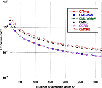

  

  MSE indices ε _C-Tyler, ε _CML-MoM, ε _CML-WMoM, and ε _CMML and bounds ε _CCRB and ε _CMCRB as function of the number M of available data vectors

  Fig. 2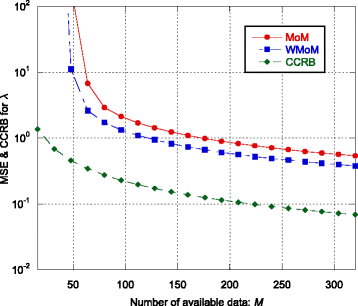

  

  MSE and CCRB on the estimate of the shape parameter λ as function of the number M of available data vectors

  Fig. 3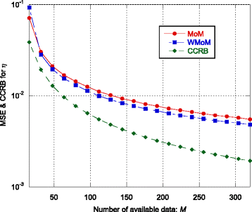

  

  MSE and CCRB on the estimate of the scale parameter η as function of the number M of available data vectors

  Fig. 4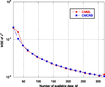

  

  MSE of the CMML estimator of σ ² and CMCRB as function of the number M of available data vectors

• 2. Estimation accuracy as function of the shape parameter λ (Figs. 5, 6, 7, and 8). Simulation parameters: ρ = 0.8, N = 16, M = 10 N, η = 1, K = 4.

  Fig. 5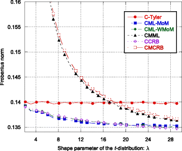

  

  The MSE indices ε _C-Tyler, ε _CML-MoM, ε _CML-WMoM, and ε _CMML and the bounds ε _CCRB and ε _CMCRB as function of the shape parameter λ

  Fig. 6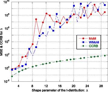

  

  MSE and CCRB on the estimate of the shape parameter λ as function of λ

  Fig. 7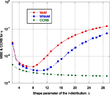

  

  MSE and CCRB on the estimate of the scale parameter η as function of the shape parameter λ

  Fig. 8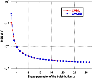

  

  MSE of the CMML estimator of σ ² and CMCRB as function of the shape parameter λ

• 3. Estimation accuracy as function of the one-lag correlation coefficient ρ (Figs. 9, 10, 11, and 12). Simulation parameters: N = 16, M = 10 N, λ = 3, η = 1, K = 4.

  Fig. 9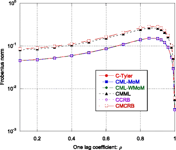

  

  The MSE indices ε _C-Tyler, ε _CML-MoM, ε _CML-WMoM, and ε _CMML and the bounds ε _CCRB and ε _CMCRB as function of the one-lag correlation coefficient ρ

  Fig. 10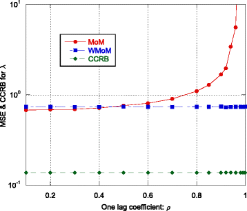

  

  MSE and CCRB on the estimate of the shape parameter λ as function of ρ

  Fig. 11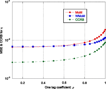

  

  MSE and CCRB on the estimate of the scale parameter η as function of ρ

  Fig. 12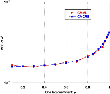

  

  MSE of the CMML estimator of σ ² and CMCRB as function of the one-lag correlation coefficient ρ

Based on the numerical analysis, we observe that:

• Regarding the scatter matrix estimation, the robust C-Tyler estimator is an “almost” efficient estimator, even if it is not the most efficient estimator for t-distributed data, in fact when λ increases, the other two estimators achieve better performance. The MSE ε _{C ‐ Tyler} is close to the CCRB especially for small λ (see Figs. 1, 5, and 9). In particular, its performance is robust, i.e., it is not affected by the value of the shape parameter λ (see Fig. 5), even if it is not efficient for large λ.

• Regarding the CMML estimator, it always achieves the CMCRB, both for the scatter matrix estimation and for the estimation of the average power (see Figs. 1, 5, 8, 9, and 12). The CMML presents a small bias on the estimation of the scatter matrix and then, ${\widehat{\boldsymbol{\Sigma}}}_{\mathrm{CMML}}$ is not a MS-unbiased estimator [9] (at least in the finite sample regime). For this reason, ε _CMML is in general slightly below the CMCRB. The loss in estimation accuracy due to the mismatch is particularly high for extremely heavy-tailed data, i.e., when λ is close to 0 (see Fig. 5). When λ → 0, the CMCRB rapidly increases while the CCRB is quite independent of λ. On the other hand, when λ → ∞, the CMCRB and the CCRB coincide, as expected, and the performance of the CMML estimator converge to that of the CML-MoM and CML-WMoM estimators.

• Quite surprisingly, even if the MoM-based estimators fail to provide an accurate estimate of λ as it increases (see Fig. 6), the MSE of the CML-MoM and CML-WMoM estimators achieve the CCRB, as shown in Fig. 5.

• Regarding the estimation of λ and η, the recursive WMoM estimator always outperforms the classical MoM estimator (see Figs. 2, 3, 7, 10, and 11), even though it does not achieve the CCRB. In particular, as shown in Fig. 10, the MSE of the WMoM is independent from the value of ρ, while this is not the case for the MSE of the classical MoM estimator. This desirable behavior of the WMoM estimator is due to the whitening operation that makes each entry of the data vectors mutually uncorrelated, as discussed in Section 3.1.

5.2 Detection performance

In this section, the detection performance of the matched LTD detector, which exploits either the CML-MoM or the CML-WMoM estimators, the mismatched Kelly’s GLRT, and the robust ANMF, that relies on the robust C-Tyler's estimator, are investigated. In particular, we analyze:

• 1. The probability of false alarm (P _FA) as function of the one-lag coefficient ρ (Fig. 13). This allows us to verify the CFAR property of the Λ _{LTD ‐ CML ‐ MoM} (Eq. (59)), Λ _{LTD ‐ CML ‐ WMoM} (Eq. (60)), Λ _Kelly (Eq. (63)), and Λ _{ANMF ‐ C ‐ Tyler} (Eq. (66)) w.r.t. the correlation shape. Simulation parameters: N = 16, M = 3 N, λ = 3, η = 1, K = 4. The detection thresholds have been set to achieve a nominal P _FA of 10⁻³.

  Fig. 13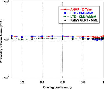

  

  Probability of false alarm vs ρ

• 2. The probability of false alarm (P _FA) as function of the shape parameter λ of the true complex t-distribution, i.e., for different spikiness levels (Fig. 14). This is important, since it highlights the CFARness of the four detectors w.r.t. the non-Gaussianity level of the data. Simulation parameters: N = 16, M = 3 N, ρ = 0.8, η = 1, K = 4. The detection thresholds have been set to achieve a nominal P _FA of 10⁻³.

  Fig. 14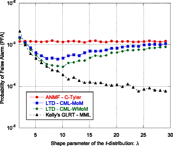

  

  Probability of false alarm vs λ

• 3. The receiver operating characteristic (ROC) curves (Fig. 15). The simulation parameters are the following: N = 16, M = 3 N, ρ = 0.8, λ = 3, η = 1, and K = 4. Moreover, $\alpha \sim CN\left(0,{\sigma}_{\alpha}^2\right)$ where ${\sigma}_{\alpha}^2$ is set to have signal to noise power ratio (SNR) equal to 3 dB.

  Fig. 15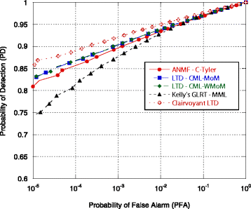

  

  Receiver operating characteristic (ROC) curves

As we can see from Fig. 13, all the analyzed detectors are CFAR with respect to ρ. Their P _FA curves are constant and close to the nominal value 10⁻³. A different behavior can be observed in Fig. 14, where the P _FA curves have been evaluated as function of λ. It can be noted that only Λ _{ANMF ‐ C ‐ Tyler} is a CFAR detector w.r.t. the data spikiness, while the P _FA of the other detectors change with λ. Finally, in Fig. 15, the ROC curves of Λ _{LTD ‐ CML ‐ MoM}, Λ _{LTD ‐ CML ‐ WMoM}, Λ _{Kelly ' s GLRT}, and Λ _{ANMF ‐ C ‐ Tyler} are shown. For the sake of comparison, we evaluated also the ROC of the clairvoyant optimum detector for the t-distributed data, i.e., the Λ _LTD in Eq. (58) where Σ, λ, and η are perfectly known. As we can see, the performance of Λ _{LTD ‐ CML ‐ MoM}, Λ _{LTD ‐ CML ‐ WMoM}, and Λ _{ANMF ‐ C ‐ Tyler} are close to that of the clairvoyant detector Λ_LTD, while Λ _{Kelly ' s GLRT} undergoes some detection loss for relatively low value of the P _FA. In particular, the fact that the performance of the robust Λ _{ANMF ‐ C ‐ Tyler} is close to the one of the matched detectors, Λ _{LTD ‐ CML ‐ MoM} and Λ _{LTD ‐ CML ‐ WMoM}, suggests that the detection loss due to the robustness is small. However, it must be highlighted again that we are considering a particular scenario in which the clutter covariance matrix is assumed to be real and full rank. Moreover, due to the high computational load of the Monte Carlo simulations, the detection performance of the proposed detectors has been evaluated only for a P _FA greater that 10⁻⁵. It would be very useful to investigate the detection performance at an operative value of P _FA, e.g., below 10⁻⁵.

6 Conclusions

This paper focused on two inference problems, the scatter matrix estimation and the adaptive detection of radar targets in complex t-distributed data. Three different approaches have been investigated and compared: the matched, the mismatched, and the robust approaches. Regarding the classical matched approach, we analyzed the performance of the CML estimator for the scatter matrix, when the shape and scale parameters are estimated through the low-complexity and suboptimal MoM method (CML-MoM) and a recursive improvement of it (CML-WMoM). We found that both the CML-MoM and the CML-WMoM estimators achieve the CCRB, while the CML-WMoM estimator outperforms the CML-MoM for the estimation of the shape and scale parameters. Then, the previous two estimators have been adapted to implement the LTD, which is the GLRT decision rule in t-distributed data. Numerical simulations show that the performance of the adaptive LTD are very close to the clairvoyant LTD detector, but it is not CFAR w.r.t. the variation of data spikyness. Regarding the mismatched approach, we proved that the CMML estimator derived under the assumption of Gaussian-distributed data converges almost surely to the true scatter matrix and to the true (t-distributed) data power, so it can be applied for inference problems that require the knowledge of these two quantities. Moreover, its efficiency with respect to the CMCRB has been shown and its performance loss with respect to the matched case discussed. The CMML estimator of the scatter matrix has been used in the “mismatched” Kelly’s GLRT. Numerical simulations proved that Kelly’s GLRT is not CFAR and presents large performance loss for small values of P _FA. Finally, the min-max robust C-Tyler scatter matrix estimator and the adaptive version of the robust NMF detector, that exploits the C-Tyler estimator, have been introduced and analyzed. In particular, our numerical results demonstrated that Tyler’s estimator is an “almost” efficient estimator w.r.t. the CCRB and its estimation accuracy is independent on the value of the shape parameter. More importantly, the resulting ANMF is CFAR w.r.t. the shape parameter, i.e., w.r.t. the level of data spikiness, and has only a small detection loss w.r.t. the clairvoyant LTD. To summarize, the results discussed in this paper show that the robust approach, thanks to its generality, robustness to misspecification, and small estimation and detection losses, seems to be the a good choice in practical applications.

References

H Krim, M Viberg, Two decades of array signal processing research: the parametric approach. IEEE Signal Process. Mag. 13(4), 67–94 (1996)
J Karhunen, J Joutsensalo, Generalizations of principal component analysis, optimization problems, and neural networks. Neural Netw. 8(4), 549–562 (1995)
O Ledoit, M Wolf, Improved estimation of the covariance matrix of stock returns with an application to portfolio selection. J. Empir. Finance 10(5), 603–621 (2003)
CD Richmond, Adaptive array signal processing and performance analysis in non-Gaussian environments. Ph.D. thesis (MIT, Cambridge, MA, 1996). Available at: https://dspace.mit.edu/handle/1721.1/11005
E Ollila, DE Tyler, V Koivunen, VH Poor, Complex elliptically symmetric distributions: survey, new results and applications. IEEE Trans. Signal Process. 60(11), 5597–5625 (2012)
KL Lange, RJA Little, JMG Taylor, Robust statistical modeling using the t distribution. J. Am. Stat. Assoc. 84(408), 881–896 (1989)
JP Romano, AF Siegel, Counterexamples in probability and statistics, Wadsworth and Brooks/Cole, Monterey, CA
S Fortunati, MS Greco, F Gini, The impact of unknown extra parameters on scatter matrix estimation and detection performance in complex t-distributed data, IEEE Workshop on Statistical Signal Processing 2016 (SSP), (IEE, Palma de Mallorca, 2016), pp 1–4. doi:10.1109/SSP.2016.7551738
S Fortunati, F Gini, MS Greco, On scatter matrix estimation in the presence of unknown extra parameters: mismatched scenario, EUSIPCO 2016, (Budapest, Hungary, 2016)
A Balleri, A Nehorai, J Wang, Maximum likelihood estimation for compound-Gaussian clutter with inverse gamma texture. IEEE Trans. Aerosp. Electron. Syst. 43(2), 775–779 (2007)
J Wang, A Dogandzic, A Nehorai, Maximum likelihood estimation of compound-Gaussian clutter and target parameters. IEEE Trans. Signal Process. 54(10), 3884–3898 (2006)
KJ Sangston, F Gini, MS Greco, Coherent radar target detection in heavy-tailed compound-Gaussian clutter. IEEE Trans. Aerosp. Electron. Syst. 48(1), 64–77 (2012)
A Younsi, M Greco, F Gini, A Zoubir, Performance of the adaptive generalised matched subspace constant false alarm rate detector in non-Gaussian noise: an experimental analysis. IET Radar Sonar Navigation 3(3), 195–202 (2009)
S Fortunati, F Gini, MS Greco, The misspecified Cramér-Rao bound and its application to the scatter matrix estimation in complex elliptically symmetric distributions. IEEE Trans. Signal Process. 64(9), 2387–2399 (2016)
S Fortunati, F Gini, MS Greco, The constrained misspecified Cramér-Rao bound. IEEE Signal Process. Lett. 23(5), 718–721 (2016)
D Tyler, A distribution-free M-estimator of multivariate scatter. Ann. Stat. 15(1), 234–251 (1987)
EJ Kelly, An adaptive detection algorithm. IEEE Trans. Aerosp. Electron. Syst. AES-22(2), 115–127 (1986)
LL Scharf, B Friedlander, Matched subspace detectors. IEEE Trans. Signal Process. 42(8), 2146–2157 (1994)
F Gini, A cumulant-based adaptive technique for coherent radar detection in a mixture of K-distributed clutter and Gaussian disturbance. IEEE Trans. Signal Process. 45(6), 1507–1519 (1997)
E Conte, A De Maio, G Ricci, Recursive estimation of the covariance matrix of a compound-Gaussian process and its application to adaptive CFAR detection. IEEE Trans. Signal Process. 50(8), 1908–1915 (2002)
F Gini, Sub-optimum coherent radar detection in a mixture of k-distributed and Gaussian clutter. IEE Proc. Part F 144(1), 39–48 (1997)
F Gini, MV Greco, A Farina, Clairvoyant and adaptive signal detection in non-Gaussian clutter: a data-dependent threshold interpretation. IEEE Trans. on Signal Processing 47(6), 1522–1531 (1999)
F Gini, MV Greco, A suboptimum approach to adaptive coherent radar detection in compound-Gaussian clutter. IEEE Trans. Aerosp. Electron. Syst. 35(3), 1095–1104 (1999)
E Ollila, DE Tyler, V Koivunen, HV Poor, Compound-Gaussian clutter modelling with an inverse Gaussian texture distribution. IEEE Signal Processing Letters 19(12), 876–879 (2012)
A Farina, F Gini, MV Greco, L Verrazzani, High resolution sea clutter data: statistical analysis of recorded live data. IEE Proc. Radar Sonar Navigation 144(3), 121–130 (1997)
R Remmer, Theory of complex functions (Springer-Verlag, New York, NY, USA, 1991)
MS Greco, F Gini, Cramér-Rao lower bounds on covariance matrix estimation for complex elliptically symmetric distributions. IEEE Trans. Signal Process. 61(24), 6401–6409 (2013)
P Stinco, MS Greco, F Gini, Adaptive detection in compound-Gaussian clutter with inverse-gamma texture. IEEE CIE International Conference on Radar 2011, 2011, pp. 434–437
MS Greco, S Fortunati, F Gini, Naive, robust or fully-adaptive: an estimation problem for CES distributions. 8-th IEEE Sensor Array and Multichannel Signal Processing Workshop (SAM 2014), 2014, pp. 457–460
JR Magnus, H Neudecker, The commutation matrix: some properties and applications. Ann. Stat. 7, 381–394 (1979)
JD Gorman, AO Hero, Lower bounds for parametric estimation with constraints. IEEE Trans. Inf. Theory 6(6), 1285–1301 (1990)
P Stoica, BC Ng, On the Cramer-Rao bound under parametric constraints. IEEE Signal Processing Letters 5(7), 177–179 (1998)
CD Richmond, LL Horowitz, Parameter bounds on estimation accuracy under model misspecification. IEEE Trans. on Signal Processing 63(9), 2263–2278 (2015)
PJ Huber, The behavior of maximum likelihood estimates under nonstandard conditions. Proc. of the Fifth Berkeley Symposium in Mathematical Statistics and Probability (University of California Press, Berkley, 1967)
H White, Maximum likelihood estimation of misspecified models. Econometrica 50, 1–25 (1982)
CC Heyde, R Morton, On constrained quasi-likelihood estimation. Biometrika 80(4), 755–61 (1993)
QH Vuong, Cramér-Rao bounds for misspecified models, Working paper 652, Division of the Humanities and Social Sciences (Caltech, 1986). Available at: https://www.hss.caltech.edu/content/cramer-rao-bounds-misspecified-models
MS Greco, S Fortunati, F Gini, Maximum likelihood covariance matrix estimation for complex elliptically symmetric distributions under mismatched conditions. Signal Process. 104, 381–386 (2014)
RA Maronna, Robust M-estimators of multivariate location and scatter. Ann. Stat. 4(1), 51–67 (1976)
F Gini, MS Greco, Covariance matrix estimation for CFAR detection in correlated heavy tailed clutter. Signal Process. 82(12), 1847–1859 (2002)
F Pascal, Y Chitour, J Ovarlez, P Forster, P Larzabal, Covariance structure maximum-likelihood estimates in compound Gaussian noise: existence and algorithm analysis. IEEE Trans. Signal Process. 56(1), 34–48 (2008)
M Skolnik, Introduction to radar systems: third edition (McGraw-Hill, New York, 2001)
CD Richmond, A note on non-Gaussian adaptive array detection and signal parameter estimation. IEEE Trans. on Signal Processing 3(8), 251–252 (1996)
NB Pulsone, RS Raghavan, Analysis of an adaptive CFAR detector in non-Gaussian interference. IEEE Trans. Aerosp. Electron. Syst. 35(3), 903–916 (1999)
F Pascal, JP Ovarlez, Asymptotic detection performance of the robust ANMF, 23rd European Signal Processing Conference (EUSIPCO), 2015, Nice, 2015, pp. 524-528
JP Ovarlez, F Pascal, A Breloy, Asymptotic detection performance analysis of the robust adaptive normalized matched filter, IEEE CAMSAP 2015, (Cancun, 2015), pp. 137-140
F Gini, JH Michels, Performance analysis of two covariance matrix estimators in compound-Gaussian clutter. IEE Proceedings Part-F 146(3), 133–140 (1999)
Competing interests
The authors declare that they have no competing interests.
Author information
Authors and Affiliations
Corresponding author
Rights and permissions
Open Access This article is distributed under the terms of the Creative Commons Attribution 4.0 International License (http://creativecommons.org/licenses/by/4.0/), which permits unrestricted use, distribution, and reproduction in any medium, provided you give appropriate credit to the original author(s) and the source, provide a link to the Creative Commons license, and indicate if changes were made.
About this article
Cite this article
Fortunati, S., Gini, F. & Greco, M.S. Matched, mismatched, and robust scatter matrix estimation and hypothesis testing in complex t-distributed data. EURASIP J. Adv. Signal Process. 2016, 123 (2016). https://doi.org/10.1186/s13634-016-0417-0
Received:
Accepted:
Published:
DOI: https://doi.org/10.1186/s13634-016-0417-0