- Research
- Open access
- Published:
Identification of piecewise affine systems based on fuzzy PCA-guided robust clustering technique
EURASIP Journal on Advances in Signal Processing volume 2016, Article number: 131 (2016)
Abstract
Hybrid systems are a class of dynamical systems whose behaviors are based on the interaction between discrete and continuous dynamical behaviors. Since a general method for the analysis of hybrid systems is not available, some researchers have focused on specific types of hybrid systems. Piecewise affine (PWA) systems are one of the subsets of hybrid systems. The identification of PWA systems includes the estimation of the parameters of affine subsystems and the coefficients of the hyperplanes defining the partition of the state-input domain. In this paper, we have proposed a PWA identification approach based on a modified clustering technique. By using a fuzzy PCA-guided robust k-means clustering algorithm along with neighborhood outlier detection, the two main drawbacks of the well-known clustering algorithms, i.e., the poor initialization and the presence of outliers, are eliminated. Furthermore, this modified clustering technique enables us to determine the number of subsystems without any prior knowledge about system. In addition, applying the structure of the state-input domain, that is, considering the time sequence of input-output pairs, provides a more efficient clustering algorithm, which is the other novelty of this work. Finally, the proposed algorithm has been evaluated by parameter identification of an IGV servo actuator. Simulation together with experiment analysis has proved the effectiveness of the proposed method.
1 Introduction
Hybrid systems are a class of dynamical systems whose behaviors are based on the interaction between discrete and continuous dynamical behaviors; in other words, at different time intervals, different dynamical behaviors can be expected from a hybrid system. Continuous and discrete dynamics are described by variables whose values are respectively chosen from a continuous and a discrete set [1]. As an example, we can refer to the dynamical behaviors of an electric heater during its OFF and ON times. Thus, the identification of hybrid systems will be very important in controlling such systems. The hybrid systems can be identified as a class of nonlinear systems. Numerous schemes have been presented for identifying nonlinear systems and the characteristics of each one have been reviewed in the literature [2, 3].
Since a general method for the analysis of hybrid systems is not available, some researchers have focused on specific types of hybrid systems. Piecewise affine (PWA) systems are one of the subsets of hybrid systems [4]. The PWA systems are defined based on the division of the state and input domains into a limited number (countable number) of polyhedral regions and the consideration of a linear/affine subsystem in every region [5]. The structure of PWA systems presents an interesting problem of system identification. In view of the universal approximation properties of PWA system maps [6, 7], these systems yield a nonlinear black-box structure. Also, considering the equivalence between PWA systems and certain classes of hybrid systems [4, 8], the identification of PWA systems constitutes a very useful step in the identification of other classes of hybrid systems.
The identification of PWA systems includes the estimation of the parameters of affine subsystems and the coefficients of the hyperplanes defining the partition of the state-input domain. Bear in mind that if the regions are not specified in advance, the association between data clustering, region, and subsystem estimation will make the identification problem very difficult. Also, if the number of subsystems is unknown, more complexity is added to the problem.
In the hybrid system identification field, the algebraic approach [9], Bayesian approach [10], bounded-error approach [11], mixed-integer programming [12], and the clustering technique [13–17] are the most important approaches, which will be enlightened in the following. For a complete overview of the presented methods and their comparison, one can refer to [1, 18, 19].
In [9], the authors have presented an algebraic-geometric solution for identifying the piecewise linear (PWL) systems. The method presented in [10] makes use of a priori knowledge about the system being identified. For this purpose, the unknown parameters are considered as random variables with their probability density functions, and the identification problem is expressed as determining a posteriori probability density function for parameters. In [11], the authors have offered a method based on MIN-PFS problem solving for a suitable number of linear complementary inequalities derived from data. The main feature of this algorithm is that it limits the identification error. In [12], the identification problem has been stated for two subclasses of PWA systems (i.e., hinging hyperplane ARX (HHARX) and Wiener PWARW (W-PWARX)) and solved by the mixed-integer linear or quadratic programs. In our paper, the data clustering is one of most important bases of proposed algorithm, which has not considered in aforementioned papers.
In general, a clustering identification method includes three steps: data clustering, parameter estimation, and region reconstruction. Obviously, the bottleneck of clustering-based approaches is the data clustering stage because the quality of parameter estimation and region reconstruction depend on the accuracy of clustering. The accuracy of clustering itself depends on three factors: (1) initialization, (2) outliers, and (3) knowing the exact number of subsystems. Since the clustering algorithms are unsupervised mostly, the initial values of cluster centers are chosen randomly; and this may lead to convergence to a local minimum. Also, the existence of outliers in data decreases the quality of many clustering algorithms considerably. Due to the unsupervised nature of clustering, the number of classes must be specified beforehand; otherwise, it must be selected through several executions of the clustering algorithm on data with different number of classes.
By presenting an approach based on regressor vector clustering in [13], authors have assigned the data to the appropriate region, and then they have determined the subsystem corresponding to each region. In this work, a modified version of k-means has been employed for clustering. In [14], a statistical clustering algorithm has been used to allocate the data to the correct regions, and the SVM has been employed to estimate the boundary hyperplane between adjacent regions. In [15], Chiu’s algorithm has been used for data clustering. The characteristic of this method is that it eliminates the outliers during the clustering process. It must be noted that in [13, 15], the regressor vector generation is based on applying a least square method on a group of adjacent data points (local dataset, or LD), which might lead to inaccurate results.
In addition, in [20], partitional clustering algorithms are considered for image segmentation because of the great similarity between segmentation and clustering, although clustering was developed for feature space, whereas segmentation was developed for the spatial domain of an image. Also in [21], a method using self-organizing map (SOM)-based spectral clustering is proposed for agriculture management. In [22], a novel distance-based feature extraction method for various pattern classification problems is introduced. Specifically, two distances are extracted, which are based on (1) the distance between the data and its intra-cluster center and (2) the distance between the data and its extra-cluster centers.
In this paper, first by using the structure of the state-input domain, that is, considering the time sequence of input-output pairs, some appropriate LDs are created. This is important, because in practice always the sequence of generation of data points is known. This is the motivation to introduce the concept of “time tag”, the label assigned to each data point to identify the sequence of them. Then using these labels, one can create some appropriate LDs. Second, the application of two novel methods, i.e., fuzzy PCA-guided robust k-means clustering algorithm [23], along with a neighborhood outlier detection algorithm [24] is studied. By customizing these methods, the performance of the existing clustering techniques is improved and usual drawbacks are solved. In fuzzy PCA-guided robust k-means clustering algorithm, there is no need to determine the cluster center, with nothing better than a random guess; therefore, poor initialization will be avoided. In addition, it should be noted that most of the clustering algorithms are not robust; this means that, repeating the execution of the clustering algorithm on the same data might be resulted in different clusters; however, in fuzzy PCA-guided robust k-means clustering, the clusters would be the same for every execution. Neighborhood outlier detection enables us to detect and eliminate the outlier before clustering. Selection of proper outliers is of crucial importance because the eliminated regressor vectors contain useful information about the problem, and most probably, improper elimination leads to imperfect results. Also, using the concept of cluster crossing curve enables us to determine the number of subsystems without any prior information. If the chosen value for the initial guess of number of subsystems was correct, the algorithm will be ended. Otherwise, the initial guess for number of subsystems will be corrected and the algorithm will be repeated. Simulation results are presented to illustrate the efficiency of the proposed method. Also, an application of the developed approach to an inlet guide vane (IGV) servo actuator is evaluated.
The remainder of the paper is organized as follows: The class of PWARX models and identification problem is stated in Section 2. In Section 3, the identification algorithm is developed, and each stage is described in detail. In Section 4, an application of the developed approach to an IGV servo actuator is assessed. Conclusions are given in Section 5.
2 Problem description
To identify the PWA systems, we need to first introduce the piecewise autoregressive exogenous (PWARX) models. In simulating the PWA systems, the PWARX models are used in order to convert a multi-input single-output system with continuous inputs to a single-input single-output system [13].
By assuming vectors u(k) ∈ R m , y(k) ∈ R p , and e(k) ∈ R p as the input, output, and error vectors, respectively, and for constant values of n 1 and n 2, the regression vector is established as follows [14]:
And the value of “n” is obtained from the following equation:
Thus, the PWARX model is defined as follows [14]:
By assuming a regression space as \( \mathcal{X}\in {\mathrm{R}}_n \), \( {\mathcal{X}}_i,\ i=1,2,\dots, s \) represents a confined convex subspace. Thus, each subspace is described asFootnote 1 [1],
where q i denotes the number of inequalities determining the ith subspace and ≼ i indicates a vector of q i dimensions with “<” and “≤” symbols as its members. Of course, it should be noted that in the PWARX models, the rules for the replacement of subsystems are determined based on the shapes of convex subspaces [13].
The number of subspaces and the variable matrices of each subsystem are indicated by s and θ i ∈ R (n + 1) × p , i = 1, 2, …, s, respectively. Subsequently, N data samples are generated as follows [14]:
Before identifying the system, certain assumptions related to problem solving must be put forward. These assumptions are as follows:
-
Assumptions (1): The number of subsystems s is a specific and predefined number.
In most cases, the structures of physical systems are such that it is possible to recognize the number of different dynamic states. Therefore, the application of Assumptions (1) will be logical and acceptable. Of course, in some cases, this estimation will not be so easy; and as a result, Assumptions (1) cannot be used. The manner of estimating the number of subsystems using the available data will be explained in Remark 2.
-
Assumptions (2): In the process of problem solving, the values of n 1 and n 2 are considered as constant and specified values.
The consideration of Assumptions (2) will be very helpful in solving the identification problem. However, we should be aware that, in practice, the values of n 1 and n 2 are seldom known, and numerous investigations have been conducted to determine the “orders” appropriately [25, 26]. In this paper, Assumptions (2) has been used in order to concentrate on various aspects of PWA systems identification without getting entangled in the complexities of “orders” estimation.
-
Assumptions (3): Knowing the time sequence of data.
Since, in practice, the data acquired from a system being identified are received sequentially within a specific time interval, each piece of data can be assigned a time tag that shows the sequence of data relative to one another in the time domain. By applying this assumption, which, in practice, is always satisfied automatically, the data can be easily divided into smaller groups with similar properties.
3 The proposed method
In view of the previously discussed matters, the identification problem is presented as follows:
Problem (1): Obtaining the parameter vectors of each subsystem (θ i , i = 1, 2, …, s) and the hyperplanes separating each two adjacent subspaces (X i , i = 1, 2, …, s) by using a specific number (r(k) , k = 1, 2, …, N) of data acquired from (3) subject to Assumptions (1) through (3).
The method presented in this paper for solving Problem (1) includes the following steps:
-
- Establishing small local datasets from the original dataset based on the chronological order of data (selecting sequential data in time domain).
-
- Calculating the parameter vectors for each local dataset.
-
- Eliminating the outlier parameter vectors by using the neighborhood outlier detection algorithm.
-
- Clustering the s-class parameter vectors by applying the fuzzy PCA-guided robust k-means clustering algorithm.
-
- Classification of original data by means of the parameter vectors corresponding to each data.
-
- Estimation of subsystems and regions by using the original data.
-
- Allocation of the original data forming the outlier parameter vectors to the correct regions, and the final estimation of subsystems and regions.
-
The flowchart of the proposed algorithm has been illustrated in Fig. 1.
Fig. 1 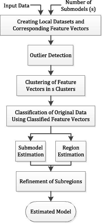
The flowchart of the proposed algorithm
-
Through mathematical Example (1), the step-by-step procedures of the proposed algorithm are described and, at each step, the details of the identification algorithm are stated.

Example (1): Consider a PWARX system with the following mathematical model:
where x(k) = [y T(k − 1) u T(k − 1) ]T, s = 3, n 1 = 0, and n 2 = 1. The input signal u(k) has been generated randomly by means of nonuniform distribution over the interval \( \overline{\mathcal{X}}=\left[-4,4.5\right] \). The PWARX system (7) with an 80-member set of noisy data ε(k) with SNR = 13 has been shown in Fig. 2. In the proposed model, the first and the third regions have the same coefficients, while they have been located in different sections of \( \overline{\mathcal{X}} \).

The PWARX system (7)
3.1 Creating local datasets
Since the subsystems of the PWARX system are linear, by considering a small number of adjacent data, a local dataset (LD) can be created [13]; on this basis, all the data of an LD can more likely belong to one region \( {\overline{\mathcal{X}}}_i \). Assumption (3) is used for this purpose. It is reasonable to consider a time tag for the data because, practically, the sequence of data generated by the system is always known and this enables the allocation of a time tag to data. Complying with this assumption makes it easy to choose the data points for the creation of LDs. For this intention, by choosing each ℓ data in sequence, an LD(Ω j ) is established. Parameter ℓ is known as the “knob” of the algorithm and its values is set by the user. Some LDs only include the data of one region (Ω1 in Fig. 2) and some others contain the data of two adjacent regions (Ω2 in Fig. 2). The first and the second types of LDs are called the “pure local dataset (PLD)” and “mixed local dataset (MLD)”, respectively [13].
The effectiveness of the clustering algorithm and, consequently, of the identification algorithm depends on the LDs. In other words, the higher the number of PLDs and the lower the number of MLDs, the higher the clustering accuracy. The number of MLDs depends on the data distribution in \( \overline{\mathcal{X}} \) and the selection of parameter ℓ (see Section 3.2.1). In case the distribution of data in \( \overline{\mathcal{X}} \) is fair, meaning that the input is excited in a way that sufficient number of data exists in each \( {\overline{\mathcal{X}}}_i \) region, and most of the data are not accumulated at the boundary between the regions, a small ratio of MLD to PLD can be achieved by an appropriate selection of parameter ℓ. It has been demonstrated in [13] that, under mild assumptions, when the number of input-output pairs (N) approaches infinity, the MLD-to-PLD ratio vanishes asymptotically. The manner of excitation of system input for the purpose of a fair distribution of data in all the regions of \( {\overline{\mathcal{X}}}_i \) is a challenging problem, which has been explored in other investigations.
3.2 Parameter vector calculation
With the consideration of ℓ > n, a parameter vector θ j corresponding to each local dataset Ω j can be calculated. For this purpose, the recursive least-squares (RLS) estimation method is used.
Computation of the least-squares estimate can be arranged in a way that the estimates obtained at time (k − 1) can be used to compute the estimates at time k. Let vector \( {\widehat{\theta}}_j\left(k-1\right) \) denote the least-squares estimate according to (k − 1) data in Ω j . By defining \( \boldsymbol{\varphi} (k)=\left[\begin{array}{c}\hfill \boldsymbol{x}(k)\hfill \\ {}\hfill 1\hfill \end{array}\right] \), it is assumed that Φ(k) = [φ T(1) … φ T(k)]T is a full rank matrix, that is, Φ T(k)Φ(k) is nonsingular for all k ≥ 0. Considering \( \widehat{\theta}(0)=0 \) and the matrix P(0) = 108 I (identity matrix I), then the vector \( {\widehat{\theta}}_j(k) \) obtains by the following recursive equations:
The components of the vector K(k) are weighting factors that tell how the correction and the previous estimate should be combined. When the data have little noise, and they have been distributed fairly and also a proper value has been chosen for ℓ, the images of vectors θ j must include s general clusters along with isolated points (henceforth called “outliers”) [13]. In fact, when the original data contain little noise, we can expect the parameter vectors θ j related to PLDs to be very similar to each other. However, under circumstance in which the existing data in an LD are from two adjacent regions, especially when the distribution of data points between two adjacent regions is discrete (boundary between regions 2 and 3 in Example (1)), the estimated parameter vectors θ j will be an outlier. We should also note that in situations where two subsystems with identical coefficients are located in two different regions (first and third subsystems in Example (1)), using the information of parameter vectors may not be sufficient for clustering them into s classes. In these conditions, the parameter vectors of these subsystems will fall next to each other and within one cluster. Resolving between these subsystems is accomplished by adding vectors m j , which indicate the average spatial position of each LD, to the parameter vector θ j . As a result, a feature vector in the form of \( {\boldsymbol{\upzeta}}_j={\left[{\theta}_j^T,{\boldsymbol{m}}_j\right]}^T \) is used for the clustering of LDs [13]. This characteristic makes it possible to resolve the subsystems that have mutual coefficients.
3.2.1 Adjusting Parameter l
In the presented approach, with the use of time tags for data and the selection of each ℓ successive data, the maximum number of outliers would amount to s − 1. In other words, in the worst case scenario, the data adjacent to the boundaries between all regions of \( {\overline{\mathcal{X}}}_{\mathrm{i}} \) and \( {\overline{\mathcal{X}}}_{\mathrm{i}+1} \) would exist in one LD and form outliers. Nevertheless, choosing a proper value for parameter ℓ will noticeably affect the performance of the detection algorithm. The relative smallness or largeness (relative to the total number of data (N)) of parameter ℓ has an advantage as well as disadvantage.
If a small value is chosen for parameter ℓ, few data will exist in each LD. The advantage of this choice is that the improper clustering of a feature vector causes a small number of data to fall in the incorrect region and, consequently, the accuracy of estimating the subsystems and regions does not diminish considerably. This choice, however, is only useful when the data are noisy just a little. In the case of too much noise, the small number of data in each LD leads to a less accurate estimation of parameter vectors θ j by the RLS method. Thus, the feature vectors ζ j will not get a proper distribution, and their clustering accuracy will diminish considerably.
On the other hand, when a large value is chosen for parameter ℓ, a more accurate estimation of parameter vectors θ j can be made by using the noisy data. Under such conditions, however, the MLDs will contain a large number of data from both the \( {\overline{\mathcal{X}}}_{\mathrm{i}} \) and \( {\overline{\mathcal{X}}}_{\mathrm{i}+1} \) regions. When the boundary between two adjacent regions is discontinuous (the boundary between regions \( {\overline{\mathcal{X}}}_2 \) and \( {\overline{\mathcal{X}}}_3 \) in Problem (1)), outliers will be generated whose positions relative to the other feature vectors are very far off. In these circumstances, the produced outliers can be eliminated by using an appropriate outlier detection algorithm. However, if the boundary between two adjacent regions is continuous (the boundary between regions \( {\overline{\mathcal{X}}}_{\mathrm{i}} \) and \( {\overline{\mathcal{X}}}_2 \) in Problem (1)), the parameter vectors θ j generated from MLDs will not be much different from those generated from PLDs; thus, these outliers cannot be eliminated by means of an outlier detection algorithm. In this case, at the clustering stage, this parameter vector is considered to belong to a class associated with one of the two adjacent regions that form the vector, while it also includes a large number of data from the other adjacent region. This leads to a lower accuracy in resolving the boundaries between regions and also in estimating the parameters of each subsystem in step 6.
Figure 3 shows the feature vector plots of the PWARX system (7) for the values of ℓ = 5, ℓ = 9, and ℓ = 13 (Fig. 3a–c, respectively) in the presence of constant noise with SNR = 14. As is illustrated, for ℓ = 5 (Fig. 3a), the feature vectors estimated by the RLS algorithm are not highly accurate. By increasing the value of parameter ℓ to 9 and 13 (Fig. 3b, c), the accuracy of the feature vectors improves significantly. It should also be noted that Fig. 3b, c do not have the same scale because the remoteness of the produced outlier (like the accuracy of the other estimated feature vectors) depends on the value of parameter ℓ, and it improves with the increase of ℓ. Also, Fig. 4a–d respectively illustrates the feature vector plots for the PWARX system (7) for noise levels of SNR = 0, 7, 14, and 21 and a constant value of ℓ = 9. As is observed, for the noise levels of SNR = 14 and 21 (Fig. 4c, d), the choice of ℓ = 9 leads to appropriate results; while by increasing the noise level (Fig. 4a, b), the estimation of feature vectors becomes less accurate and, therefore, the value of parameter ℓ must be increased in order to improve the results. However, it should be noted that if a large value is chosen for ℓ (in order to suppress the noise effects), it will lead to a lower accuracy in resolving the boundaries between regions and also estimating the parameters of each subsystem. Based on the above explanations, we conclude that a suitable value can be achieved for parameter ℓ through a tradeoff between the quality of estimation of parameter vectors θ j from noisy data, quality of delineation of the boundary between regions, and also the quality of estimation of each subsystem’s parameters.

The feature vector plots of the PWARX system (7) for the values of a ℓ = 5, b ℓ = 9, and c ℓ = 13 in the presence of constant noise with SNR = 14

The feature vector plots for the PWARX system (7) for noise levels of SNR = a 0, b 7, c 14, and d 21, and a constant value of ℓ = 9
The advantage of using a time tag to form the LDs is the independence of the number of outliers from parameter ℓ; this means that, with the increase of ℓ, the number of outliers does not necessarily increase (Fig. 3). This is while in the methods presented in [13, 15], the LDs are selected in such a way that the number of outliers depends on the value of parameter ℓ. As a result, selecting a large value for ℓ (in order to suppress the noise effects) leads to an increase in the number of outliers. Therefore, in these approaches, the value of ℓ has to be chosen accurately; while it is difficult to exactly determine the most suitable value for this parameter.
3.3 Outlier detection
As was mentioned in Section 3.2.1, when parameter vector θ j has been calculated by using a MLD, one outlier might be produced. Considering the incorrect positioning of this outlier relative to the other feature vectors, the clustering process will run into a problem. Thus, in the proposed method, an outlier detection step prior to clustering has been considered. In this procedure, all the feature vectors estimated in the previous step are handed over to an appropriate outlier detection algorithm to determine the outliers. For this purpose, the neighborhood outlier detection algorithm [24] has been used in this paper. A brief description of this algorithm is provided below.
Consider the nonempty finite sets of U and G which respectively include all the feature vectors and attributes. For each ζ j ∈ U and H ⊆ G, the neighborhood of ζ j in subspace H is defined as \( {n}_H^q\left({\boldsymbol{\upzeta}}_j\right) \)
where q is called the neighborhood parameter. A distance metric is a distance function that maps two points to a space of nonnegative integers. As an example, we can use the Euclidean distance of points in an (n + 2)-dimensional space (G = g 1, g 2, …, g n + 2),
where f(ζ j , g i ) indicates the value of data x in the ith dimension.
After calculating the neighborhood \( \left({n}_H^q\right) \) for all the existing data in U, by considering a neighborhood parameter q g for each feature g ∈ G, the distance between two data (ζ j and ζ k ) in feature g is determined as follows:
Then, the value difference metric (VDM) is calculated from the following equation:
In the next step, the neighborhood-based object outlier factor (NOOF) for each data ζ ji ∈ U is determined by using the VDM N values
Suppose that a threshold value μ has been given; for each ζ j ∈ U, if F(ζ j ) > μ, then ζ j is called a neighborhood-based outlier in U. More details of the algorithm can be observed in [24].
The parameters affecting the performance of the outlier detection algorithm include the neighborhood parameter \( q=\left\{{q}_{g_1},{q}_{g_2},\dots, {q}_{g_{n+2}}\right\} \) corresponding to each feature G = {g 1, g 2, …, g n + 2} and also the threshold value μ. The value of neighborhood parameter \( {q}_{a_i} \) is determined with regard to the value of feature g i . Choosing small values for q g reduction of \( {n}_g^{q_g}\left({\boldsymbol{\upzeta}}_j\right) \). This means that there would be fewer data adjacent to data ζ j along feature g.
Following the establishment of feature vectors in Section 3.2, the outlier detection algorithm with q = {2, 5, 1} and μ = 0.9 is used to remove the outlier resulting from the MLD. Figure 5a, b respectively show the feature vectors (marked with circle) along with the outlier (marked with square) and the feature vectors after the elimination of the outlier. As is observed, after removing the outlier, the data distribution is well formed and the clustering operation can be implemented with a high precision.

a The feature vectors (marked with circle) along with the outlier (marked with square) and b the feature vectors after the elimination of the outlier
Remark (1): When the data of an MLD include the data of two \( {\overline{\mathcal{X}}}_{\mathrm{i}} \) and \( {\overline{\mathcal{X}}}_{\mathrm{i}+1} \) regions with a discontinuous boundary, the feature vector corresponding to this MLD will emerge as an outlier. The necessity of eliminating the outliers was discussed in Section 3.3. However, it should be noted that the removal of an outlier means the removal of the original data corresponding to that outlier. This causes the loss of some valuable information about the system. Since the original data corresponding to outlier feature vectors usually include the data existing at the boundaries between regions \( {\overline{\mathcal{X}}}_{\mathrm{i}} \), their elimination reduces the accuracy of detecting such boundaries. Thus, a refinement step has been considered at the end of the algorithm for the reassignment of original data corresponding to outliers.
3.4 Clustering the feature vectors
After eliminating the outliers by means of the algorithm presented in Section 3.3, it is time to cluster the remaining feature vectors. There are various clustering algorithms (for a description of these different approaches, refer to [27, 28]). However, it should be noted that some of these algorithms suffer from two drawbacks: (1) poor initialization and (2) noisy data. To overcome these two problems, in this paper, the fuzzy PCA-guided robust k-means clustering algorithm [23] has been used. The three main advantages of this method over the other approaches are
-
Using this algorithm eliminates the need to randomly determine the class centers and thus ensures that poor initialization will not lead to the convergence of response to a local optima.
-
By exploiting the frameworks of the fuzzy and PCA methods, a noise-resistant approach is created.
-
By mapping the data to a space of higher dimension using the kernel function, it is possible to establish a nonlinear decision boundary.
In the following, the fuzzy PCA-guided robust k-means clustering algorithm [23] will be briefly described.
Choose the initial value of responsibility weights b i , i = 1, 2, …, n + 2 as b i = 1 and choose the noise sensitivity wright β (the recommended value is β = 1) and the termination condition ε. Set s to the initial guess for number of clusters.
Calculate the normalized kernel matrix as follows:
where I n is n × n unit matrix, \( \boldsymbol{b}=\left({b}_1^{\alpha },\dots, {b}_{n+2}^{\alpha}\right) \), θ is the weighting exponent used to estimate fuzzy memberships (a recommended value is α = 2), h is the n-dimensional vector whose all elements are 1, W = {w ij } is the kernel PCA-guided k-means matrix whose element is w ij = ϕ w (ζ i )T ϕ w (ζ j ) for each ζ = [ζ1 ζ2 ….. ζ n + 2], and ϕ w is a nonlinear transformation to higher dimensional space are centered as Φ w S b T h = 0 where Φ w = (ϕ w (ζ1), …., ϕ w (ζ n + 2)).
Derive J s − 1 = (j 1, …, j s − 1) by calculating the eigenvectors corresponding to s − 1 largest eigenvalues of B α/2 WB α/2, where B is a diagonal matrix whose ith diagonal element is b i . Then, set j s as follows:
Then, the responsibility criterion λ i , i = 1, …, n + 2 and penalty weight γ is calculated as follows:
Then, b i is updated as below:
If \( { \max}_i\left|{b}_i^{NEW}-{b}_i^{OLD}\right|<\varepsilon \), then output connectivity matrix C or P = {p ij },
Otherwise, return to step 2.
Here, p ij is large only when samples i and j are in the same cluster, and none of them is a noise sample; the noise samples have small connectivity with the other samples. A potential approach to assessment of cluster structure is distance-sensitive ordering of samples [29]. After distance-sensitive ordering, cluster structure is shown in the diagonal block structure of connectivity matrix. To find cluster boundaries, [29] proposed “cluster crossing.” Cluster crossing is the sum along the antidiagonal direction in connectivity matrix and takes a minimum at the cluster boundaries between clusters (shown with “x” marker in Fig. 6b). Figure 6a–c shows the connectivity matrix C, cluster crossing curve, and the classified feature vector for Example (1).

a Connectivity matrix C, b cluster crossing curve, and (c) the classified feature vector for Example (1)
As is observed in Fig. 6a, b, by using the diagonal block structure of the connectivity matrix or the cluster crossing curve, the boundaries between classes can be delineated. The results of applying the fuzzy PCA-guided robust k-means clustering algorithm in the clustering of the feature vectors in Example (1) have been illustrated in Fig. 6c.
3.5 Original dataset classification
Following the clustering of feature vectors ζ, the original data can be classified by using the correspondence between each feature vector ζ j and a number of original data. In fact, each feature vector ζ j corresponds to one LD Ω j . By using the same correspondence, the original data associated with each \( {\overline{\mathcal{X}}}_i,\ \mathrm{i}=1,2,\dots, \mathrm{s} \) can be determined. The classified data of Example (1) have been shown in Fig. 7a. Due to the removal of the outlier feature vector, which includes some of the data near the boundary between the \( {\overline{\mathcal{X}}}_2 \) and \( {\overline{\mathcal{X}}}_3 \) regions (Remark (1)), no data exists in the vicinity of the boundary between these regions. Figure 7b illustrates the boundary between the \( {\overline{\mathcal{X}}}_1 \) and \( {\overline{\mathcal{X}}}_2 \) regions more accurately. We can see that only two data from the \( {\overline{\mathcal{X}}}_1 \) region have been incorrectly placed in the \( {\overline{\mathcal{X}}}_2 \) region.

a, b The classified data of Example (1)
3.6 Estimation of subsystems and subregions
Now by using the existing data in \( {\overline{\mathcal{X}}}_i,\ \mathrm{i}=1,2,\dots, \mathrm{s} \), the subsystems and regions can be estimated. The RLS method with formulation (8) is employed to estimate the subsystems. The following estimations are obtained for the subsystems of Example (1):
It is observed that the obtained subsystems (21) are very close to those of the PWARX system (7).
After getting an estimation for the subsystems, it is time to obtain an estimation for the unknown regions \( {\left\{{\mathcal{X}}_i\right\}}_{i=1}^s \). Since all the sets of \( {\mathcal{X}}_i \) are polyhedral and convex, for each pair of \( {\mathcal{X}}_i \) and \( {\mathcal{X}}_j \) with i ≠ j, there will be a separating hyperplane expressed by equation \( {\boldsymbol{M}}_{ij}^{\mathrm{T}}\boldsymbol{x}={m}_{ij} \), and for it, we will have [13],
where M ij is the normal vector to the hyperplane \( {\boldsymbol{M}}_{ij}^{\mathrm{T}}\boldsymbol{x}={m}_{ij} \) and m ij is the bias. To estimate \( {\boldsymbol{M}}_{ij}^{\mathrm{T}}\boldsymbol{x}={m}_{ij} \), we can use the support vector machine (SVM) [30] with linear kernel. Since “holes” are not accepted in the model, the multicategory classification approach can be employed to create the \( {\mathcal{X}}_i \) regions. For this purpose, the multicategory support vector machine (M-SVM) method can be used. For more details in this regard, one can refer to [13, 22].
Finally, the \( {\mathcal{X}}_i \) regions for Example (1) are estimated as follows:
By examining the above results more closely, we can see that, due to the removal of the outlier feature vector, the beginning and end of the region boundary have not been delineated with a high precision. Thus, an additional step is suggested for using the data that form the outlier feature vector.
3.7 Refinement
In this step, by using a simple rule, the original data corresponding to the outlier feature vector are returned to their correct regions. For this purpose, the estimated subsystems in are used; so that for each outlier’s regression vector x, estimation error error i corresponding to the ith subspace \( {\mathcal{X}}_i \) can be computed using (3) and (4) as belows:
where y sys(x) is the real output corresponding to input x and \( {\boldsymbol{y}}_{{\mathrm{est}}_i}\left(\boldsymbol{x}\right) \) is the output of the ith estimated subsystem for input x. In this step, the real output of each data is compared with the outputs of the estimated subsystems and then the data is assigned to a region with least error. In this way, by using a simple method, the original data forming the outlier feature vector can be assigned to the correct \( {\mathcal{X}}_i \) regions. Following this procedure, the subsystems and regions are re-estimated, as in Section 3.6. The results of the refinement step for Example (1) have been shown in Eq. (25) and Fig. 8. We can see that by adding the refinement step, the accuracy of estimating the \( {\mathcal{X}}_i \) regions improves considerably.

Classified data points (circles, crosses, triangles)
Remark (2): As was stated in Assumption (1), the number of subsystems s is assumed to be known. When s is unspecified, its value should be estimated based on the data. Cluster crossing is the sum along the antidiagonal direction in the connectivity matrix with a bandwidth \( \tilde{m} \) and takes a minimum at the cluster boundaries between clusters, i.e., each cluster forms a “peak” in the cluster-crossing curve [23]. By finding “peaks” and “valleys” in the curve, we can visually capture the cluster structures in the connectivity matrix. When s is unspecified, its value should be estimated based on the data. To achieve this, the cluster-crossing curve can be used. For this purpose, by considering s i , i = 2, 3, …, the clustering algorithm is executed and the cluster-crossing curve is plotted for each value of s. In these conditions, the cluster-crossing curve for s i ≤ s actual follows a pattern of peaks and valleys (with a number equal to s i ). However, for s i > s actual, the pattern of the cluster-crossing curve loses its regularity. Thus, an estimation of the number of subsystems can be obtained.
4 Identification of an IGV servo actuator
In this section, the application of proposed method to identify an IGV servo actuator is evaluated. A gas turbine engine includes a compressor with multiple rows of rotor blades spaced between multiple rows of stator vanes to gradually compress air for delivery to a combustor. Many gas turbine engines include a first stage of inlet guide vanes that are variable in order to change the angle of each guide vane.
The IGV servo actuator controls the position of the inlet guide vanes of the industrial gas turbine system. The actuator provides highly accurate position control. The actuator is a double-acting design that will close the guide vane on loss of electrical signals. Optimum control of the inlet guide vane requires that the actuator accurately and quickly track the demand signals transmitted by the control. The IGV actuator has been designed to provide output forces that exceed the opening and closing requirements. The additional margin helps ensure that the system moves rapidly even under service conditions where the actuator has been contaminated or worn.
The IGV actuator is controlled by an electronic servo-control system, which compares the demanded and actual actuator positions. The control system modulates the input current signal to the electrohydraulic servo valve to minimize the positioning system error. The available electronic servo-control system is a kind of Direct Current (DC) motor that uses a switching PI controller with different sets of gains and is used to track the desired angular velocity. The controller gains varies in the different range of electrical current i(t). The aforementioned system is shown in Fig. 9.

The identified IGV servo system
The model of a DC motor is described by the following continuous-time state-space equations:
where v(t) is the input voltage, ω(t) is the angular velocity of the rotor, and T o is the external torque which is applied to the rotor with inertia of J. L, R, and B, represent winding leakage inductance, armature resistance, and the frictional coefficient, respectively. Also, k t and k v denote torque and back emf constant, respectively.
A switching PI controller is used to track the desired angular velocity ω ref(t). So, by defining e ω (t) = ω ref(t) − ω(t), the input voltage of the motor is equal to
Also by using the trapezoidal rule for approximating the integral, the input voltage at time t = kT s is given by
where n 1 = 1, n 2 = 2, y(k − 1) = v(k − 1), and x(k) = [v(k − 1) e ω (k − 1) e ω (k − 2)]T. So, the identification problem consists of finding variable matrices of each subsystem θ i = [1 a i b i ]T for PWARX systems (29) and estimating the regions of electrical current X i . The available data is related to an electronic servo-control system under a sinusoidal T o (t) with variable ω ref(t), and the data were sampled at T s = 0.001 s. In this case, a sinusoidal T o was estimated to be as
Also, ω ref(t) which is related to a particular industrial application sets as Fig. 10.

Angular velocity of the rotor
This data set consists of enough data of the electrical current, input voltage in proposed operating conditions which is plotted in Fig. 11b, c, respectively. Also, changes in regions over time are shown in Fig. 11a. There is a driver software that comes with the electronic servo-control system which provides the output data for user. The identification problem consists of finding the gains of the three PI controllers and estimating the regions of the electrical current.

Changes in current (b) and voltage (c) of the electronic servo-control system with respect to changes in regions (a) from experimental data
In order to determine the gains of the PI controller, we need to estimate the parameters of each subsystem. In the following, with the use of the proposed algorithm, estimated parameters of each subsystem and regions are obtained as Table 1. The value of parameter ℓ was selected to 7, but, it is noticeable that we can choose ℓ in a wide range without affecting the results. Also, Fig. 12 illustrates the connectivity matrix and cluster crossing curve of classified feature vectors. As it can be seen, by choosing s = 3, diagonal block structure of this matrix enables us to cluster data points carefully. It should be noted that s = 1, 2, 3 and 4 have been chosen as initial guess to cluster the feature vectors. Finally, Fig. 13 shows the real and estimated angular velocity of the electronic servo-control system. For this purpose, using the mathematical model of an electronic servo-control system, and by applying the working condition of the identified servo system, the estimated angular velocity of the motor is assessed for controller gains in Table 1. Figure 13 shows that the identification is done perfectly, and the real and estimated angular velocities have the same behavior (the error percentage between real and estimated angular velocities is about 2.34% in 10 s).

a Connectivity matrix and b cluster crossing curve of classified feature vectors for IGV servo actuator

Real and estimated angular velocity of the electronic servo-control system
5 Conclusions
In this paper, an effective method for identification of piecewise affine system is proposed. This method uses the clustering of feature vectors that consist of parameter vectors corresponding to local datasets and average spatial position of each one. Since, in practice, the data acquired from a system being identified are received sequentially within a specific time interval, each piece of data can be assigned a label, time tag, which shows the sequence of data relative to one another in the time domain. Also, since the subsystems of the PWARX system are linear, by considering a small number of data in a specified time interval, a LD can be created. Then, using RLS algorithm, a parameter vector is calculated for each LD. By adding the average spatial position of each LD to corresponding parameter vector, a feature vector is created. This modification makes it possible to resolve the subsystems that have mutual coefficients.
Because some LD contains data points from two adjacent regions, some outlier feature vectors are produced. So, by using the neighborhood outlier detection method, these ill feature vectors are eliminated. Then, fuzzy PCA-guided robust k-means clustering algorithm is implemented for feature vectors clustering. This clustering method uses a specific predetermined value for membership degree of each data point, so there is no need to use some initial centers for clusters. This modification avoids getting trapped in local minima. Furthermore, cluster crossing curve enables us to estimate the number of subsystems. This is a useful trick, especially in the case that we have not enough information about system. After that, a refinement stage is considered to improve the subsystem and region estimation. In this stage, the ambiguity concerned with outliers is solved. By integrating all these desirable characteristics, a practical identification algorithm is created.
This paper mainly concerns the possibility to improve the clustering of feature vectors because as mentioned earlier, the bottleneck of clustering-based approaches is feature vectors clustering. The effectiveness of the proposed method is investigated through a mathematical and industrial model. Results show the ability of the proposed method in identification of industrial systems in the presences of noise. Also, the main drawbacks of the earlier clustering-based methods are solved in this paper.
Notes
It is assumed that each subspace satisfies the relations of \( {\mathcal{X}}_i\ne \varnothing\ \forall i\ \in\ \left\{1,2,\dots, s\right\} \), \( {\mathcal{X}}_i{\displaystyle \cap}\kern.2em {\mathcal{X}}_j=\varnothing \forall i,\kern.2em j\in \left\{1,2,\dots, s\right\},i\ne j \), and \( {{\displaystyle \cup}}_{i=1}^s{\mathcal{X}}_i=\mathcal{X} \).
References
S Paoletti, AL Juloski, G Ferrari-Trecate, R Vidal, Identification of hybrid systems a tutorial. Eur. J. Control. 13(2-3), 242–260 (2007)
A Juditsky, H Hjalmarsson, A Benveniste, B Delyon, L Ljung, J SjÖberg, Q Zhang, Nonlinear black-box models in system identification: mathematical foundations. Automatica 31(12), 1725–1750 (1995)
J Sjöberg, Q Zhang, L Ljung, A Benveniste, B Delyon, P-Y Glorennec, H Hjalmarsson, A Juditsky, Nonlinear black-box modeling in system identification: a unified overview. Automatica 31(12), 1691–1724 (1995)
WPMH Heemels, BD Schutter, A Bemporad, Equivalence of hybrid dynamical models. Automatica 37, 1085–1091 (2001)
ED Sontag, Nonlinear regulation: the piecewise linear approach. IEEE Trans. Autom. Control 26(2), 346–358 (1981)
JN Lin, R Unbehauen, Canonical piecewise-linear approximations. IEEE Trans. Circuits Syst. I, Fundam. Theory Appl. 39(8), 697–699 (1992)
L Breiman, Hinging hyperplanes for regression, classification, and function approximation. IEEE Trans. Inf. Theory 39(3), 999–1013 (1993)
A Bemporad, G Ferrari-Trecate, M Morari, Observability and controllability of piecewise affine and hybrid systems. IEEE Trans. Autom. Control 45(10), 1864–1876 (2000)
R Vidal, S Soatto, Y Ma, SS Sastry, An algebraic geometric approach to the identification of a class of linear hybrid systems, in Proceedings 42nd IEEE Conference on Decision and Control, vol. 1, 2003, pp. 167–172
AL Juloski, S Weiland, WPMH Heemels, A bayesian approach to identification of hybrid systems. IEEE Trans. Autom. Control 50, 1502–1533 (2005)
A Bemporad, A Garulli, S Paoletti, A Vicino, A bounded-error approach to piecewise affine system identification. IEEE Trans. Autom. Control 50, 1567–1580 (2005)
J Roll, A Bemporad, L Ljung, Identification of piecewise affine systems via mixed-integer programming. Automatica 40(1), 37–50 (2004)
G Ferrari-Trecate, M Muselli, D Liberati, M Morari, A clustering technique for the identification of piecewise affine systems. Automatica 39, 205–217 (2003)
H Nakada, K Takaba, T Katayama, Identification of piecewise affine systems based on statistical clustering technique. Automatica 41, 905–913 (2005)
Z Lassoued, K Abderrahim, An experimental validation of a novel clustering approach to PWARX identification. Eng. Appl. Artif. Intell. 28, 201–209 (2014)
Z Lassoued, K Abderrahim, A Kohonen neural network based method for PWARX identification, in 11th IFAC International Workshop on Adaptation and Learning in Control and Signal Processing, 2013, pp. 742–747
Z Lassoued, K Abderrahim, Comparison study of some PWARX system identification methods, in 17th International Conference on System Theory, Control and Computing (ICSTCC), 2013, pp. 291–296
J Roll, Local and piecewise affine approaches to system identification (Department of Electrical Engineering, Linkoping University, Linkoping, 2003)
AL Juloski, S Paoletti, J Roll, Recent techniques for the identification of piecewise affine and hybrid systems, in Current Trends in Nonlinear Systems and Control, 2006, pp. 79–99
J Quintanilla-Domínguez, B Ojeda-Magaña, A Marcano-Cedeño, MG Cortina-Januchs, A Vega-Corona, D Andina, Improvement for detection of microcalcifications through clustering algorithms and artificial neural networks. EURASIP J. Adv. Signal Process. 2011(1), 1 (2011)
K Tasdemir, C Wirnhardt, Neural network-based clustering for agriculture management. EURASIP J. Adv. Signal Process. 2012(1), 1–3 (2012)
C-F Tsai, W-Y Lin, Z-F Hong, C-Y Hsieh, Distance-based features in pattern classification. EURASIP J. Adv. Signal Process. 2011(1), 1 (2011)
K Honda, A Notsu, H Ichihashi, Fuzzy PCA-guided robust k-means clustering. IEEE Trans. Fuzzy Syst. 18, 67–79 (2010)
Y Chen, D Miao, H Zhang, Neighborhood outlier detection. Expert Syst. Appl. 37, 8745–8749 (2010)
L Ljung, System identification—theory for the user (Prentice-Hall, Upper Saddle River, 1999)
T Soderstrom, P Stoica, System identification (Prentice-Hall, Inc, Hemel Hempstead, 1989)
RO Duda, PE Hart, Pattern classification and scene analysis (Wiley, New York, 1973)
AK Jain, RC Dubes, Algorithms for clustering data (Prentice Hall College Div, New Jersey, 1988)
C Ding, X He, Linearized cluster assignment via spectral ordering, in Proceedings of the twenty-first international conference on Machine learning, 2004, pp. 233–240
V Vapnik, Statistical learning theory (Wiley, New York, 1998)
Authors’ contributions
All authors read and approved the final manuscript.
Competing interests
The authors declare that they have no competing interests.
Author information
Authors and Affiliations
Corresponding author
Rights and permissions
Open Access This article is distributed under the terms of the Creative Commons Attribution 4.0 International License (http://creativecommons.org/licenses/by/4.0/), which permits unrestricted use, distribution, and reproduction in any medium, provided you give appropriate credit to the original author(s) and the source, provide a link to the Creative Commons license, and indicate if changes were made.
About this article

Cite this article
Khanmirza, E., Nazarahari, M. & Mousavi, A. Identification of piecewise affine systems based on fuzzy PCA-guided robust clustering technique. EURASIP J. Adv. Signal Process. 2016, 131 (2016). https://doi.org/10.1186/s13634-016-0427-y
Received:
Accepted:
Published:
DOI: https://doi.org/10.1186/s13634-016-0427-y