Spectrum sensing based on cumulative power spectral density

Abstract

This paper presents new spectrum sensing algorithms based on the cumulative power spectral density (CPSD). The proposed detectors examine the CPSD of the received signal to make a decision on the absence/presence of the primary user (PU) signal. Those detectors require the whiteness of the noise in the band of interest. The false alarm and detection probabilities are derived analytically and simulated under Gaussian and Rayleigh fading channels. Our proposed detectors present better performance than the energy (ED) or the cyclostationary detectors (CSD). Moreover, in the presence of noise uncertainty (NU), they are shown to provide more robustness than ED, with less performance loss. In order to neglect the NU, we modified our algorithms to be independent from the noise variance.

1 Introduction

Due to an increasing demand of wireless devices and the limitation of natural spectrum resources, the cognitive radio (CR) has been introduced to optimize the use of the available spectrum [1]. In CR network, primary (PU) and secondary (SU) users can share the same bandwidth. PU is a licensed user, whereas SU is an opportunistic user. To avoid any interference with the PU’s signal, SU can only be active when PU is idle. Therefore, SU should continuously monitor PU status (active or idle).

Many factors (such as low signal to noise ratio (SNR), shadowing, channel fading, etc.) lead to a situation where SU is no longer able to correctly diagnose the status of the PU. To overcome this problem, new techniques for cooperative spectrum sensing (CSS) have been proposed [2, 3]. In the CSS context, several SUs cooperate to reach a decision on the presence of the PU signal; a fusion center (FC) should make the final decision. We can distinguish two schemes of CSS: the soft and the hard combining schemes. In the soft combining scheme, each SU sends its own measured test statistic to the FC who performs a linear combination of all received test statistics and compares the result to a threshold. With the hard combining scheme, each SU compares its own test statistic to a predefined threshold, makes his decision on the PU status, and sends it to the FC, where a final decision is made by combining the decisions of all the SUs using a predefined strategy (such as OR, AND, or a majority strategy).

In the literature, many techniques have been proposed to perform test statistics. Most known methods are energy detection, cysclostationary detection, and waveform detection. The last one requires perfect information about the PU signal [3, 4]. Hence, the use of this method is limited to the case of cooperative relationship between PUs and SUs.

Due to its simplicity and the fact that no prior information about the PU signal is required, the energy detector (ED) is widely used in spectrum sensing. ED consists of measuring the energy of the received signals and comparing it to a predefined threshold based on the known noise variance. Therefore, ED requires an accurate estimation of the noise variance; otherwise, we can face a SNR-wall problem, where the ED becomes incapable to made a robust decision about the PU status, even with a very large observation time [5, 6]. However, many studies have been proposed to enhance the energy detector (ED) performance and to overcome its limitations [5, 7–9].

The cyclostationary features detection (CSD) [10] is also widely used in spectrum sensing. CSD requires the knowledge of the cyclic frequencies of the PU, in addition to a long observation time and computing efforts. In [11], a cooperative CSD is proposed, where each SU performs a single cyclic-frequency detection and sends his decision to a FC to make the final decision. The authors of [12] analyzed theoretically the performance of the algorithm proposed in [11] in multi-path and log-normal channels. In [13], a blind CSD is proposed. This detector performs the spectrum sensing without the knowledge of the cyclic frequencies.

Although energy and cyclostationary detectors are widely used in the field of spectrum sensing, various other methods are also proposed [14–16]. The goodness of fit (GoF) algorithm introduced in [14] compares the empirical distribution of the received samples to a known distribution of the noise (when PU is idle). If the empirical distribution is not compatible with the known distribution of the noise then the PU signal exists. To enhance the performance, [15] extends the algorithm of [14] by using the square of the received samples instead of the samples themselves.

By assuming the oversampling aspect of the baseband received signal (i.e., number of samples per symbols N _s ≥2), the autocorrelation for a non-zero lag only vanishes when the PU signal is absent and the channel is only occupied by a white noise [16]. The corresponding test statistic combines linearly the autocorrelation measures for different non-zero lags before making a decision on the PU status. The performance of this algorithm increases with N _s .

In this paper, we propose new spectrum sensing detectors based mainly on the cumulative sum of the power spectral density (PSD) of the received signal¹. It is known that the PSD of a white noise is flat. However, PSD losses this property with an oversampled PU signal. If the PU is absent, the cumulative sum of the received signal PSD has a close shape to a straight line. Whereas, a curved shape is obtained when PU exists.

To enhance the robustness of our contribution, hard and soft combining schemes are introduced. In those two schemes, the spectrum is divided into two parts: at first, the negative frequency points are considered while the second part deals with the positive frequency points. Hence, two test statistics are calculated based on the cumulative PSD of each part, and they are then combined according to the considered scheme.

The false alarm and detection probabilities are evaluated analytically under Gaussian and Rayleigh fading channels. Our detectors are compared to ED and CSD [8, 16]. Our detectors present a better performance than the energy detector, even at N _s =2 samples per symbol, where the CSD detector provides a poor performance relatively to ED. Furthermore, our detectors are less sensitive to the noise uncertainty than ED. In particular, we demonstrate that our detectors can be modified to become independent from the noise variance. This case represents an important advantage in real scenarios.

The rest of this paper is organized as follows. In Section 2, the system model and the spectrum sensing hypothesis are presented, in addition to an overview of the PSD and its estimation. Our proposed detectors based on the cumulative sum of the PSD are discussed in Section 3. Section 4 provides an analytic study on the statistical distributions of the test statistics as well as the calculus of the false alarm and detection probabilities. In Section 5, the probability of detection over Rayleigh flat-fading channel is provided. The numerical results of our detectors will be presented in Section 6. The effects of the noise uncertainty problem on our detectors are shown in Section 7. To overcome the noise uncertainty problem, this section presents modified versions of our detectors which are independent of the noise variance. At the end, a conclusion and perspective section of our work is provided.

2 System model and generality

The spectrum sensing consists in making a decision on the presence of PU in a bandwidth of interest (BoI). The PU baseband signal, s(n), can be modeled as follows:

$$ s(n)=\sum_{m} b_{m} g(n-{mN}_{s})=s_{p}(n)+ {js}_{q}(n) $$

(1)

b _m are the symbols to be transmitted; g(n) is the shaping window; N _s satisfies the Nyquist criterion; $N_{s}=\frac {F_{s}}{B}\geq 2$ samples per symbol (sps), where F _s is the sampling frequency and s _p (n) and s _q (n) are respectively the real and imaginary parts of s(n). s(n) has a bandwidth B and an even power spectral density (PSD). s(n) is assumed to be complex-valued zero mean unknown deterministic² signal [11, 12, 17–19].

The presence/absence of PU can be presented in a classic Bayesian detection problem. Under H ₀, the PU is absent, whereas under H ₁ PU exists.

$$ \left\{ \begin{array}{l} H_{0}: y(n)=w(n) \\ H_{1}: y(n)=hs(n)+w(n) \end{array} \right. $$

(2)

where h is the complex channel gain. w(n) is $\mathcal {N}(0,\sigma _{w}^{2})$, where $\mathcal {N}(m,V)$ stands for a normal distribution of a mean m and a variance V. Further, w(n)=w _p (n)+jw _q (n) is an i.i.d complex circular symmetric, i.e.,

E[w ²(n)]=0 and the real part, w _p (n), and the imaginary part, w _q (n), of w(n) are independent Gaussian processes with equal variance.

$$\begin{array}{*{20}l} E\left[w_{p}^{2}(n)\right]&=E\left[w_{q}^{2}(n)\right]=\frac{\sigma_{w}^{2}}{2} \end{array} $$

(3)

Where $\sigma _{w}^{2}=E[|w(n)|^{2}]$ and E[.] stands for the expectation. Without loss of generality, we assume that s(n) is a unit power signal. In this case, the signal to noise ratio (SNR), γ, is defined as follows:

$$ \gamma=\frac{|h|^{2}}{\sigma_{w}^{2}} $$

(4)

A wrong decision about the channel status can affect either the PU transmission or the efficient use of the channel. In fact, a missed detection can cause a harmful interference by the transmission of the SU in the same band of the PU. A false alarm, however, decreases the profit of the opportunity of the channel. Therefore, the probability of detection (p _d ) should be increased as much as possible, by keeping the probability of false alarm (p _fa ) low. Neyman-Person’s detection method consists in a trade-off between a high p _d and a low p _fa .

2.1 Power spectral density

The power spectral density (PSD), P _x (k), of a wide sense stationary signal x(n) is the Fourier transform ($\mathcal {FT}$) of its autocorrelation function, r _xx (m) [20]:

$$\begin{array}{*{20}l} r_{xx}(m)&=E\left[x(n)x^{*}(n-m)\right] \end{array} $$

(5)

$$\begin{array}{*{20}l} P_{x}(k)&=\mathcal{FT}\left\{ r_{xx}(m) \right\} \end{array} $$

(6)

Thanks to the whiteness of the noise, the autocorrelation function of w(n) becomes

$$ r_{ww}(m)=E\left[w(n)w^{*}(n-m)\right]=\sigma_{w}^{2}\delta(m) $$

(7)

where δ(m) is Kronecker’s function. Based on Eq. (7), the PSD of the white noise, P _w (k), becomes real, even and constant over the frequency band [−B;B], with an amplitude $\sigma _{w}^{2}$. It is obvious that the cumulative sum of the PSD becomes a straight line, with a slope $\sigma _{w}^{2}$.

According to the model (1), s(n) is a cyclostationary signal characterized by its cyclic spectral density (CSD), $S_{s}^{\alpha }(k)$ [13, 18]:

$$\begin{array}{*{20}l} S_{s}^{\alpha}(k)&=\mathcal{FT}\!\left\{R(\alpha,m)\right\} \,=\,{\lim}_{N \longrightarrow \infty}\frac{1}{N}S_{N}\left(\!k-\frac{\alpha}{2}\!\right)S_{N}^{*}\left(k+\frac{\alpha}{2}\right) \end{array} $$

(8)

where α is a cyclic frequency of s(n), $S_{N}(k)=\mathcal {FT}\left \{s(n)\right \}$ is the $\mathcal {FT}$ of N received samples of s(n)³ and R(α,m) is the cyclic autocorrelation function of s(n) and can be defined as [18, 19]:

$$ R(\alpha,m)=\! {\lim}_{N \longrightarrow \infty}\frac{1}{N}\sum\limits_{n=-\frac{N}{2}+1}^{\frac{P}{2}} s(n)s^{*}(n-m) \exp\left(-j2\pi\alpha \frac{n}{N}\right) $$

(9)

According to Eq. (10), the PSD, P _s (k), of s(n) can be evaluated for null cyclic frequency (i.e., α=0),

$$\begin{array}{*{20}l} P_{s}(k)=S_{s}^{0}(k)&=\mathcal{FT}\left\{R(0,m)\right\}={\lim}_{N \longrightarrow \infty}\frac{1}{N}|S_{N}(k)|^{2} \end{array} $$

(10)

Due to the fact that the PU signal is not an i.i.d. signal (i.e. R(0,m) is not a Kronecker’s function), then its PSD, P _s (k), should be not constant on [−B;B]. Based on this fact, the distinguish between H ₀ and H ₁ can be realized using the shape of the cumulative sum of PSD.

2.2 Estimation of the power spectral density

The PSD of the received signal y(n) can be estimated by its periodogram as follows [20]:

$$ \hat{P}_{y}(k) = \frac{1}{N}|Y(k)|^{2} $$

(11)

where Y(k) is the discrete Fourier transform (DFT) of the signal y(n) with N samples:

$$ Y(k)=\sum\limits_{n=\frac{N}{2}-1}^{\frac{N}{2}} y(n) \exp{\left(-j2\pi k \frac{n}{N}\right)} $$

(12)

Therefore, the estimated PSD of the signal is related to the modulus of its DFT.

Since w(n) is a circular symmetric process, then its DFT W(k) becomes also a zero mean circular symmetric process [21–23].

3 Cumulative power spectral density-based detector

The cumulative power spectral density (CPSD), ψ _y (k), of the received signal y(n) is defined, over a frequency interval I=[v;l] ∀k∈I as follows :

$$ \psi_{y}(k)=\sum\limits_{u=v}^{k} \hat{P}_{y}(u), $$

(13)

where $\hat {P}_{y}(u)$ is the estimated PSD of y(n) using Eq. (11). Unlike ED, which makes the sum of energy on all frequency points of PSD, CPSD makes the sum of the energy on a given frequency points interval. The sense of variation of CPSD will be tested in order to make a decision on the PU signal existence as detailed below.

The expected value of ψ _w (k),v≤k≤l, of w(n) can be found as follows:

$$\begin{array}{*{20}l} E[\psi_{w}(k)]&= \frac{1}{N}\sum\limits_{p=v}^{k} E\left[|W(p)|^{2}\right] \\ &= \frac{1}{N}\sum\limits_{p=v}^{k} \sum\limits_{n=1}^{N}\sum\limits_{m=1}^{N} E\left[{\vphantom{\exp{\left(-j2\pi(n-m)\frac{p}{N}\right)}}}w(n)w^{*}(m) \right.\\ &\left.\ \ \ \exp{\left(-j2\pi(n-m)\frac{p}{N}\right)}\right] \\ &= \frac{1}{N}\sum\limits_{u=v}^{k} \underbrace{\sum\limits_{n=m=1}^{N}E\left[|w(n)|^{2}\right]}_{=N\sigma_{w}^{2}}] \\ &=\frac{1}{N}(k-v+1)N\sigma_{w}^{2} \\ &=(k-v+1)\sigma_{w}^{2} \end{array} $$

(14)

The last value shows that ψ _w (k) increases linearly on the frequency interval [v,l] with k till its highest value $(l-v+1)\sigma _{w}^{2}$.

Let us define the normalized CPSD, Γ(k), of y(n) by

$$ \Gamma(k)=\frac{\psi_{y}(k)}{(l-v+1)\sigma_{w}^{2}} $$

(15)

Due to this normalization, under H ₀, Γ(k) still increase to one. Thus, under H ₀ and thanks to the flat PSD of w(n), the shape of Γ(k) becomes closed to a straight line R(v,l;k).

$$ R(v,l;k)=\frac{k-v+1}{l-v+1} $$

(16)

Under H ₁, this constraint is not satisfied, since the PSD of s(n) is not a constant, and Γ(k) has higher values than the one obtained under H ₀ due to the additional power of s(n).

Figures 1 and 2 show Γ(k) under H ₀ and H ₁ for rectangular and raise-cosine (roll-off factor = 0.5) pulse shaping filters respectively, for various values of N _s and different SNR. The signal modulation is 16-QAM, and the number of used samples is N=10000. As shown in Figs. 1 and 2, the gap between the normalized CPSD shape under H ₁ and that under H ₀ increases with the SNR for both considered pulse shaping filters. In addition, the non-linearity of the CPSD shapes grows with N _s . Therefore, we define a test statistic T as the difference between Γ(k) and the reference straight line R(v,l;k). Accordingly, we introduce two detectors:

• 1. T _p : This detector is based on the CPSD, Γ _p (k), of $\hat {P}_{y}(k)$ for positive frequency points

  Fig. 1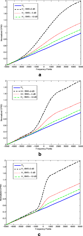

  

  The normalized CPSD shapes for N=10000 samples and several values of N _s and SNR: rectangular pulse-shaping filter. a N _s = 2 sps. b N _s = 4 sps. c N _s = 8 sps

  Fig. 2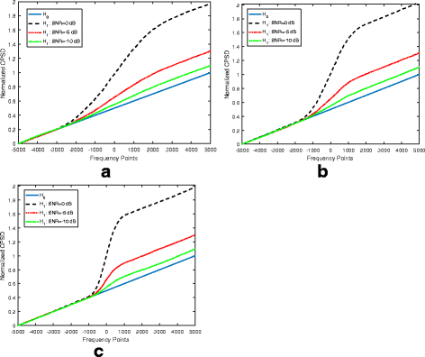

  

  The normalized CPSD shapes for N=10000 samples and several values of N _s and SNR: raised cosine pulse-shaping filter. a N _s = 2 sps. b N _s = 4 sps. c N _s = 8 sps

  (i.e.,$\ 1\leq k \leq \frac {N}{2}$), in this case, the corresponding CPSD, ψ _p (k), is defined as follows:

  $$\begin{array}{*{20}l} \psi_{p}(k)=\sum\limits_{u=1}^{k} \hat{P}_{y}(u) \end{array} $$

  (17)

  Accordingly, the normalized CPSD, Γ _p (k) becomes

  $$\begin{array}{*{20}l} \Gamma_{p}(k)&=\frac{\psi_{p}(k)}{\left(\frac{N}{2}-1+1\right)\sigma_{w}^{2}}\\ &=\frac{2}{N\sigma_{w}^{2}}\sum\limits_{u=1}^{k} \hat{P}_{y}(u) \\ &=\frac{2}{N^{2}\sigma_{w}^{2}}\sum\limits_{u=1}^{k}|Y(u)|^{2} \end{array} $$

  (18)

  and the reference straight line $R\left (1,\frac {N}{2};k\right)$ is obtained by

  $$\begin{array}{*{20}l} R\left(1,\frac{N}{2};k\right)=\frac{k-1+1}{\frac{N}{2}-1+1}=\frac{2k}{N} \end{array} $$

  (19)

  T _p detector aims at finding the difference between Γ _p (k) and the corresponding reference shape $R\left (1,\frac {N}{2};k\right)$:

  $$\begin{array}{*{20}l} T_{p}&=\sum\limits_{k=1}^{\frac{N}{2}} \left(\Gamma_{p}(k)-R\left(1,\frac{N}{2};k\right)\right) \\ T_{p}&=\sum\limits_{k=1}^{\frac{N}{2}} \left(\Gamma_{p}(k)-\frac{2k}{N}\right) \\ &=\sum_{k=1}^{\frac{N}{2}} \Gamma_{p}(k)-\frac{N+2}{4} \end{array} $$

  (20)

• 2. T _a : This detector is based on the CPSD of all frequencies of y(n) (i.e., $-\frac {N}{2}+1\ \leq \ k \leq \ \frac {N}{2}$), similarly to T _p :

$$\begin{array}{*{20}l}T_{a} &=\sum\limits_{k=-\frac{N}{2}+1}^{\frac{N}{2}} \left(\Gamma_{a}(k)-R\left(-\frac{N}{2}+1,\frac{N}{2};k\right)\right) \\ &=\sum_{k=-\frac{N}{2}+1}^{\frac{N}{2}} \Gamma_{a}(k)-\frac{N+1}{2} \end{array} $$

(21)

Where Γ _a (k) can be found as follows:

$$ \Gamma_{a}(k)=\frac{1}{N^{2}\sigma_{w}^{2}}\sum\limits_{u=-\frac{N}{2}+1}^{k}|Y(u)|^{2} $$

(22)

3.1 Proposed combining detectors

In this section, two combining detectors are proposed. The first proposed detector, T _or , aims at exploiting all the frequency points of the signal y(n), by applying two test statistics: the first one tests the shape of the CPSD for positive frequency points (which is T _p ), and T _n tests the CPSD shape of the CPSD of the symmetric of P _y (k) part standing for the negative frequency points (i.e.,$\ -\frac {N}{2}+1\ \leq \ k\ \leq \ 0$).

$$\begin{array}{*{20}l} T_{n}&=\sum\limits_{k=1}^{\frac{N}{2}} \left(\Gamma_{n}(k)-R\left(1,\frac{N}{2};k\right)\right) \\ &=\sum_{k=1}^{\frac{N}{2}} \Gamma_{n}(k)-\frac{N+2}{4} \end{array} $$

(23)

where Γ _n (k) in this case is given by

$$\begin{array}{*{20}l} \Gamma_{n}(k)=\frac{2}{N^{2}\sigma_{w}^{2}}\sum_{u=1}^{k} \left|Y(-u+1)\right|^{2} \end{array} $$

(24)

Since P _s (k) is symmetric and deterministic (as s(n) is deterministic) and the components of W(k) are i.i.d. (as it is shown in Section 4.1.1); therefore T _p and T _n become independent and have same mean and variance.

Once T _p and T _n make their own decisions, T _or , acting as hard cooperative detector, processes those two decisions using an OR rule.

$$ T_{or}=OR(D_{T_{p}},D_{T_{n}}) $$

(25)

where $D_{T_{p}}$ and $D_{T_{n}}$ are the detection results of T _p and T _n respectively.

The second proposed cooperative detector, T _av , performs the average, P _av , between the positive frequency PSD and the symmetric of the negative frequency PSD of the received signal. CPSD is then performed on P _av . The averaging process smooth the PSD, since P _s (k) is symmetric, and the components of $\hat {P}_{w}(k)$ are independent as shown in Section 4.

$$ P_{av}(k)=\frac{P_{y}(k)+P_{y}(-k+1)}{2}; \ \ \ \ \ \ \ \ 1\ \leq\ k\ \leq\ \frac{N}{2} $$

(26)

T _av can be considered as a soft combining detector of T _p and T _n .

$$\begin{array}{*{20}l} T_{av}&=\sum\limits_{k=1}^{\frac{N}{2}} \Gamma_{av}(k)-R\left(1,\frac{N}{2};k\right) \\ &=\sum\limits_{k=1}^{\frac{N}{2}} \Gamma_{av}(k)-\frac{N+2}{4} \end{array} $$

(27)

where the first term of the previous equation becomes

$$ \Gamma_{av}(k)=\frac{2}{N\sigma_{w}^{2}}\sum\limits_{u=1}^{k} P_{av}(u) $$

(28)

4 Statistical analysis

Distributions of test statistics are essential in order to find analytically the probability of false alarm p _fa and the detection probability p _d . T _p and T _a have the same statistical distribution since W(k) is i.i.d. and S(k) is deterministic as s(n) is assumed to be deterministic. In the following, we develop the distribution of T _p under H ₀ and H ₁ over a Gaussian channel, where the channel effect h is assumed to be constant. Similarly, the distribution of T _a can be found. T _or made its decision by applying the logical OR on the decisions of T _p and T _n which have the same distribution.

4.1 False alarm and detection probabilities of T _p

The distribution of T _p depends on ${\sum \nolimits }_{k=1}^{\frac {N}{2}} \Gamma _{p}(k)$ as presented in Eq. (20). A simplification of the term ${\sum \nolimits }_{k=1}^{\frac {N}{2}} \Gamma _{p}(k)$ can be obtained as follows (see Appendix 1):

$$\begin{array}{*{20}l} \sum\limits_{k=1}^{\frac{N}{2}} \Gamma_{p}(k)&=\frac{2}{N^{2}\sigma_{w}^{2}}\sum\limits_{k=1}^{\frac{N}{2}} \sum\limits_{u=1}^{k}|Y(u)|^{2} \\ &=\frac{2}{N^{2}\sigma_{w}^{2}}\sum\limits_{k=1}^{\frac{N}{2}} \left(\frac{N}{2}-k+1\right)|Y(k)|^{2} \end{array} $$

(29)

4.1.1 False alarm probability of T _p

Under H ₀, the test statistic T _p is only related to the noise w(n). Using Eq. (29), T _p can be written as follows:

$$\begin{array}{*{20}l} T_{p}&=\sum\limits_{k=1}^{\frac{N}{2}} \left[\frac{2}{N^{2}\sigma_{w}^{2}}\left(\frac{N}{2}-k+1\right)\left|W(k)\right|^{2}-R\left(1,\frac{N}{2};k\right)\right]\\ &=\sum\limits_{k=1}^{\frac{N}{2}}\left[\Gamma_{p}(k)-R\left(1,\frac{N}{2};k\right)\right] \end{array} $$

(30)

Being the discrete Fourier transform of a white noise w(n), W(k) asymptotically follows a normal distribution since it is the sum of independent terms. It is known that two Gaussian variables are independent if they are uncorrelated [22]. As E[W(k)W ^∗(k−m)]=E[W(k)]E[W ^∗(k−m)]=0 (see Appendix (2)), then W(k) becomes i.i.d.

Being the sum of independent terms and according to the central limit theorem, the distribution of T _p tends towards $\mathcal {N}(\mu _{0},V_{0})$ under H ₀. In this case, the probability of false alarm $p_{fa}^{p}$ of T _p can be found as follows:

$$ p_{fa}^{p}=Q\left(\frac{\lambda-\mu_{0}}{\sqrt{V_{0}}}\right) $$

(31)

where Q(.) is the Q-function ⁴, and λ is the threshold of comparison. Since $E\left [|W(k)|^{2}\right ]\ =N\sigma _{w}^{2}$ and based on Eq. (30), we can evaluate μ ₀ as follows:

$$\begin{array}{*{20}l} \mu_{0}&=E[T_{p} ] \\ &=\frac{2}{N^{2}\sigma_{w}^{2}}\sum_{k=1}^{\frac{N}{2}} \left(\frac{N}{2}-k+1\right)E\left[|W(k)|^{2}\right]-\frac{N+2}{4} \\ &=0 \end{array} $$

(32)

In this case, the variance, V ₀, of T _p becomes (see Appendix 4)

$$\begin{array}{*{20}l} V_{0}&=E\left[T_{p}^{2}\right]=\frac{(N+2)(N+1)}{6N} \end{array} $$

(33)

4.1.2 Probability of detection of T _p

Under H ₁, Y(k)=hS(k)+W(k), then Eq. (29) becomes as follows:

$$ \Gamma_{p}(k)=\frac{2}{N^{2}\sigma_{w}^{2}}\sum\limits_{k=1}^{\frac{N}{2}} \left(\frac{N}{2}-k+1\right)\left|hS(k)+W(k)\right|^{2} $$

(34)

Since S(k) is deterministic and the terms of W(k) are independent, the distribution of T _p under H ₁ tends also towards $\mathcal {N}(\mu _{1},V_{1})$. In this case, the probability of detection $p_{d}^{p}$, of T _p can be found as follows:

$$ p_{d}^{p}=Q\left(\frac{\lambda-\mu_{1}}{\sqrt{V_{1}}}\right) $$

(35)

μ ₁ and V ₁ should be evaluated in order to find $p_{d}^{p}$. Under H ₁, |Y(k)|² becomes

$$\begin{array}{*{20}l} |Y(k)|^{2}&=Y(k)Y^{*}(k) \\ &=|hS(k)|^{2}+|W(k)|^{2}+2Re\{hS(k)W^{*}(k)\} \end{array} $$

(36)

where hS(k)=DFT{hs(n)} and Re{X} is the real part of X. The mean value of T _p under H ₁ can be found as follows (see Appendix 3):

$$ \mu_{1}=b\gamma $$

(37)

where $b=\frac {2}{N^{2}}\sum _{k=1}^{\frac {N}{2}}(\frac {N}{2}-k+1)|S(k)|^{2}$, and γ is the SNR as defined by Eq. (4).

Under H ₁, the variance V ₁ is given by the following equation (see Appendix 5):

$$\begin{array}{*{20}l} V_{1}&\,=\,V_{0}+\frac{8\gamma}{N^{3}}\sum_{k=1}^{\frac{N}{2}} \left(\frac{N}{2}-k+1\right)^{2}|S(k)|^{2} &=V_{0}+c\gamma \end{array} $$

(38)

where $c=\frac {8}{N^{3}}{\sum \nolimits }_{k=1}^{\frac {N}{2}} \left (\frac {N}{2}-k+1\right)^{2}|S(k)|^{2}$.

T _a is based on similar idea to T _p , but it covers the N frequency points instead of just positive frequency points ($\frac {N}{2}$ points). Since W(k) is i.i.d. and S(k) is deterministic, then by following the same process for $p_{fa}^{p}$ and $p_{d}^{p}$, the probability of false alarm $p_{fa}^{a}$ and the probability of detection $p_{d}^{a}$ of the detector T _a can be found as follows:

$$\begin{array}{*{20}l} p_{fa}^{a}=Q\left(\frac{\lambda-\mu_{0}^{a}}{\sqrt{V_{0}^{a}}}\right) \end{array} $$

(39)

$$\begin{array}{*{20}l} p_{d}^{a}=Q\left(\frac{\lambda-\mu_{1}^{a}}{\sqrt{V_{1}^{a}}}\right) \end{array} $$

(40)

where $\mu _{0}^{a}=0$; $V_{0}^{a}=\frac {N}{3}+\frac {1}{2}+\frac {1}{6N}$; $\mu _{1}^{a}=b_{a}\gamma$, where $b_{a}=\frac {1}{N^{2}}\sum _{k=1}^{N}(N-k+1)|S(k)|^{2}$, and $V_{1}^{a}=V_{0}^{a}+c_{a}\gamma$, where $c_{a}=\frac {2}{N^{3}}\sum _{k=1}^{N} (N-k+1)^{2}|S(k)|^{2}$.

4.2 Probabilities of T _or

T _or applies the OR rule between the decisions of T _p and T _n , then T _or can be considered as a hard cooperative detector of these two detectors. Since T _p and T _n are independent and have the same statistics as we defined previously, the probability of false alarm $p_{fa}^{or}$ and the probability of detection $p_{d}^{or}$ of T _or can be found as follows [2]:

$$\begin{array}{*{20}l} p_{fa}^{or}&=1-\left(1-p_{fa}^{p} \right)^{2} \end{array} $$

(41)

$$\begin{array}{*{20}l} p_{d}^{or}&=1-\left(1-p_{d}^{p} \right)^{2} \end{array} $$

(42)

4.3 Probabilities of T _av

T _av can be developed following similar steps as Eq. (30).

$$\begin{array}{*{20}l} T_{av}&=\frac{2}{N^{2}\sigma_{w}^{2}}\sum\limits_{k=1}^{\frac{N}{2}}\left(\frac{N}{2}-k+1\right)\frac{|Y(k)|^{2}+|Y(-k+1)|^{2}}{2}\\ &\quad-\frac{N+2}{4} \end{array} $$

(43)

Under H ₀, Y(k)=W(k), then T _av becomes the sum of independent terms. Based on CLT, T _av asymptotically follows $\mathcal {N}(\mu _{0}^{av},V_{0}^{av})$ under H ₀.

Under H ₁, Y(k)=hS(k)+W(k) and S(k) is deterministic, so T _av is still following a normal distribution: $\mathcal {N}(\mu _{1}^{av},V_{1}^{av})$ under H ₁.

The probability of false alarm, $p_{fa}^{av}$, and detection, $p_{d}^{av}$, of T _av are expressed as follows:

$$\begin{array}{*{20}l} p_{fa}^{av}=Q\left(\frac{\lambda-\mu_{0}^{av}}{\sqrt{V_{0}^{av}}}\right) \end{array} $$

(44)

$$\begin{array}{*{20}l} p_{d}^{av}=Q\left(\frac{\lambda-\mu_{1}^{av}}{\sqrt{V_{1}^{av}}}\right) \end{array} $$

(45)

Since W(k) is i.i.d. and P _s (k) is even, $\mu _{0}^{av},V_{0}^{av}$, $\mu _{1}^{av}$, $V_{1}^{av}$ can be found by following similar steps to μ ₀, V ₀, μ ₁ and V ₁, we can find that $\mu _{0}^{av}=\mu _{0}$, $V_{0}^{av}=\frac {V_{0}}{2}$, $\mu _{1}^{av}=\mu _{1}$, and $V_{1}^{av}=\frac {V_{1}}{2}$.

The theoretical and the simulated ROC curves of proposed detectors are with good agreement as shown in Figs. 3 a, b. Simulations were done under following conditions: 16-QAM modulation, γ=−12 dB, N=1000 samples, and N _s =4 sps.

Fig. 3

Simulated vs. analytical results over Gaussian channel for rectangular and raised-cosine pulse-shaping filters. a Rectangular pulse-shaping filter. b Raised-cosine pulse-shaping filter: roll-off factor = 0.5

As shown in Fig. 3 a, T _av is the most efficient detector for both considered shaping filters. For the simulations of Section 6 under Gaussian channel, only T _av and T _or are compared to other well-known detectors. The rest of simulations in this paper are done with a rectangular pulse-shaping filter.

5 Probability of detection over Rayleigh fading channel

In this section, we derive the detection probability over the Rayleigh flat-fading channel. The false alarm probability remains the same since it is independent of the channel gain h. The distribution of the SNR, γ, in a Rayleigh channel is given by [21]:

$$\begin{array}{*{20}l} f_{\gamma}(\gamma)=\frac{1}{\bar{\gamma}}\exp{\left(-\frac{\gamma}{\bar{\gamma}}\right)} \end{array} $$

(46)

where $\bar {\gamma }$ is the average SNR.

Over a Rayleigh channel, the probability of detection, p _dr , is found by averaging the probability of detection, p _dg under Gaussian channel with respect to f _γ (γ).

$$\begin{array}{*{20}l} p_{dr}=\int_{0}^{+\infty}p_{dg}f_{\gamma}(\gamma)d\gamma \end{array} $$

(47)

Concerning our detectors, T _p , T _a , and T _av , their detection probabilities over Rayleigh fading channel can be derived similarly, since they have a similar probability of detection: $p=Q(\frac {\lambda -\delta \gamma }{V_{H_{0}} + \beta \gamma })$, where δ, $V_{H_{0}}$, and β are constants.

Hereinafter, we only derive $p_{dr}^{p}$, the detection probability of T _p over a Rayleigh channel. Once $p_{dr}^{p}$ is derived, $p_{dr}^{a}$ and $p_{dr}^{av}$, the probability of detection of T _a and T _av , can be easily found.

Using Eqs. (35), (46), and (47), $p_{dr}^{p}$ can be expressed as follows:

$$\begin{array}{*{20}l} p_{dr}^{p}&=\frac{1}{\bar{\gamma}}\int_{0}^{+\infty}Q \left(\frac{\lambda-\mu_{1}}{\sqrt{V_{1}}}\right)\exp{\left(-\frac{\gamma}{\bar{\gamma}}\right)}d\gamma \end{array} $$

(48)

The above integral does not have an analytic solution. Therefore, Taylor series of the first order are used to approximate the argument of the Q-function, $g(\gamma)=\frac {\lambda -b\gamma }{\sqrt {V_{0}+c\gamma }}$, around γ ₀=λ/b as follows (see Appendix 6):

$$\begin{array}{*{20}l} g_{1}(\gamma)& = g(\gamma_{0})+g'(\gamma_{0})(\gamma - \gamma_{0}) \\ &=g'(\gamma_{0})(\gamma-\gamma_{0}) \end{array} $$

(49)

where g ₁(γ) is the first-order Taylor series approximation of g(γ).

The approximation of $p_{dr}^{p}$, $\hat {p}_{dr}^{p}$ is given by :

$$\begin{array}{*{20}l} \hat{p}_{dr}^{p}=\frac{1}{\bar{\gamma}}\int_{0}^{+\infty} Q\Bigg(\theta(\gamma-\gamma_{0})\Bigg) \exp{\left(-\frac{\gamma}{\bar{\gamma}}\right)} d\gamma \end{array} $$

(50)

With $\theta =g'(\gamma _{0})=-\frac {b}{\sqrt {V_{0}+c\lambda /b}}$. According to [24], we can find

$$\begin{array}{*{20}l} \int \exp{(qx)}Q(px)dx&=\frac{1}{q}\left[{\vphantom{-\exp{\left(\frac{q^{2}}{2p^{2}}\right)}Q\left(px-\frac{q}{p}\right)}}\exp{(qx)}Q(px)\right.\\ &\left.\quad-\exp{\left(\frac{q^{2}}{2p^{2}}\right)}Q\left(px-\frac{q}{p}\right)\right] \end{array} $$

(51)

Using Eq. (51) and the fact that Q(−x)=1−Q(x), the integral of Eq. (50) becomes

$$\begin{array}{*{20}l} \hat{p}_{dr}^{p}&=Q(-\theta\gamma_{0})+\exp{\left(\frac{1}{2\theta^{2}\bar{\gamma}^{2}}-\frac{\gamma_{0}}{\bar{\gamma}}\right)}Q\left(\theta \gamma_{0} -\frac{1}{\theta \bar{\gamma}}\right) \end{array} $$

(52)

For the approximation $\hat {p}_{dr}^{a}$, of $p_{dr}^{a}$, it can be found by replacing the number of samples N/2 used in T _p by N used in T _a . Similarly to $\hat {p}_{dr}^{p}$,the approximation $\hat {p}_{dr}^{av}$ of $p_{dr}^{av}$ can be derived as follows:

$$\begin{array}{*{20}l} \hat{p}_{dr}^{av}&=Q\left(-\theta_{av}\gamma_{0}\right)\\ &\quad+\exp{\left(\frac{1}{2\theta_{av}^{2}\bar{\gamma}^{2}}-\frac{\gamma_{0}}{\bar{\gamma}}\right)}Q\left(\theta_{av} \gamma_{0} -\frac{1}{\theta_{av} \bar{\gamma}}\right) \end{array} $$

(53)

where $\theta _{av}=-\frac {b}{\sqrt {V_{0av}+\frac {c\lambda }{2b}}}$.

γ ₀ is not modified in the expression of $\hat {p}_{dr}^{av}$, since T _p and T _av have the same mean under H ₁.

The detection probability of T _or under Gaussian channel is a non-linear combination of the probability of detection of T _p and T _n . Over a Rayleigh channel, the fading coefficient, h, is the same for T _p and T _n , $p_{dr}^{or}$ of T _or becomes

$$\begin{array}{*{20}l} p_{dr}^{or}&=\frac{1}{\hat{\gamma}}\int_{0}^{\infty} \left(1-\left(1-p_{d}^{p}\right)^{2}\right)\exp{\left(-\frac{\gamma}{\bar{\gamma}}\right)}d\gamma \\ &= \frac{2}{\bar{\gamma}}\int_{0}^{\infty} Q\left(\frac{\lambda-b\gamma}{\sqrt{V_{0}+c\gamma}}\right)\exp{\Bigg(-\frac{\gamma}{\bar{\gamma}}\Bigg)}d\gamma \\ &\quad-\frac{1}{\bar{\gamma}}\int_{0}^{\infty} Q^{2}\left(\frac{\lambda-b\gamma}{\sqrt{V_{0}+c\gamma}}\right)\exp{\Bigg(-\frac{\gamma}{\bar{\gamma}}\Bigg)}d\gamma \end{array} $$

(54)

As there is no analytic solution of Eq. (54), we solve it in numerical way.

In Fig. 4, analytical results are very closed to simulation results. T _av and T _or both achieve the best performance among the proposed detectors, thus they will be compared to the well-known ED and CSD under Rayleigh channel.

Fig. 4

Simulated vs. analytical results over Rayleigh fading channel, N _s =3 sps

6 Performance evaluation

In this section, we compare the performance of our detectors to that of the energy detector (ED) [8] and the cyclostationary detector (CSD) [10], under Gaussian and Rayleigh channels. Throughout the upcoming simulations, A 16-QAM baseband-modulated PU signal with a rectangular pulse-shaping filter is considered.

6.1 Performance analysis over Gaussian channel

Figure 5 presents the ROC curves under a Gaussian channel of various numbers of samples per symbol N _s . Simulations are done using N=1500 samples and γ=−12 dB. According to that figure, the performance increases with N _s . For the limiting case, i.e., when N _s =2 sps, CSD shows a poor performance relatively to T _av , T _or , and ED, while T _av outperforms all other detectors. However, T _av and T _or outperform ED and CSD for different values of N _s .

Fig. 5

ROC curves of our proposed detectors comparing to ED and CSD for various N _s , SNR of -12 dB and N=1500 samples. a N _s = 2 sps. b N _s = 4 sps. c N _s = 8 sps

Figure 6 shows the variation of the probability of detection with respect to SNR for a constant p _fa =0.1. The number of samples is fixed N=1000 samples, and various values are assigned for N _s . T _av and T _or reach higher probabilities of detection than ED and CSD for similar SNR and different values of N _s . In addition, increasing N _s leads to enhancing the performance of T _or , T _av , and CSD. For example, T _av reaches p _d =0.9 at SNR ≃−7 dB for N _s =2 sps, while the same probability of detection is reached for SNR ≃−9 dB and SNR ≃−10 dB at N _s =4 sps and N _s =8 sps respectively.

Fig. 6

Variation of the probability of detection in terms of SNR for N=1000 samples, a constant p _fa =0.1, and various values of N _s . a N _s = 2 sps. b N _s = 4 sps. c N _s = 8 sps

6.2 Performance analysis over Rayleigh channel

Figure 7 shows the ROC curves under Raleigh fading channel for N _s =4 and N _s =8 sps, with N=1000 samples and an average SNR of −5 dB.

Fig. 7

ROC curves over Rayleigh fading channel for a) N _s = 4 sps and b N _s = 8 sps for N=1000 samples and average SNR =−5 dB

Over Rayleigh fading channel, T _av and T _or are still outperforming ED and CSD. The same fading suffered by the negative and the positive frequency parts of PSD affects the performance of our detectors. This fact makes the performances of ED and CSD closed to the proposed detectors, as shown in Fig. 7, where the gap of performance among our detectors, ED and CSD becomes smaller comparing it to a Gaussian channel.

6.3 Complexity analysis

According to Eq. (29), T _p needs $\frac {N}{2}$ operations to obtain |Y(k)|² and $\frac {N}{2}$ multiplication operations to evaluate the product $\left (\frac {N}{2}-k+1\right)|Y(k)|^{2}$. Moreover, T _p performs N addition operations: $\frac {N}{2}$ operations to calculate $\left (\frac {N}{2}-k+1\right)$, $\frac {N}{2}-1$ operations to compute the overall sum and, at the end, one addition operation is required to subtract $\frac {N+2}{4}$. Furthermore, to compute the Y(k), we need Nlog ₂(N) operations using the fast Fourier transform (FFT) algorithm. The overall number of operations needed by T _p is $\mathcal {C}(T_{p})$:

$$ \mathcal{C}(T_{p})=N\left(2+\text{log}_{2}(N)\right) $$

(55)

To obtain the decision of T _or , we have to previously find T _p and T _n . Since those two test statistics have the same complexity, therefore, the complexity of T _or becomes the double of that of T _p except for the calculus of the FFT which should be evaluated once. Then the required number of operations of T _or , $\mathcal {C}(T_{or})$, becomes

$$ \mathcal{C}(T_{or})=N\left(4+{log}_{2}(N)\right) $$

(56)

For T _av , we can find the corresponding number of operations, $\mathcal {C}(T_{or})$, similarly to T _or :

$$ \mathcal{C}(T_{av})=N\left(3+{log}_{2}(N)\right) $$

(57)

To compare the complexity of our detectors to that of ED and CSD, we should emphasize that ED needs N operations of multiplication and N−1 for addition:

$$ \mathcal{C}(ED)=2N-1 $$

(58)

For CSD, the corresponding number of operations, $\mathcal {C}(CSD)$, can be derived as follows [25]:

$$\begin{array}{*{20}l} \mathcal{C}(CSD)&=(N_{s}-1)N(L+1)+4(N_{s}-1)L^{2} \\ &\ \ \ \ +8(N_{s}-1)^{3}+6(N_{s}-1)^{2}+2(N_{s}-1) \end{array} $$

(59)

where L is an odd number and stands for the length for the unit window used in the detection process of CSD [10].

According to Eqs. (56) and (57), the complexity T _or and T _av is independent of the number of samples per symbol N _s , contrary to CSD where the complexity depends on N _s as shown in Eq. (59). As shown previously, increasing the oversampling rate leads to obtain a robust performance for CSD, T _or and T _av , while the performance of ED is not affected by the oversampling rate.

Figure 8 shows the number of samples and the complexity of the various detectors in terms SNR for a target (p _fa ;p _d )=(0.1;0.9) under a Gaussian channel. As shown in Fig. 8 a, T _or and T _av need a number of samples less than that of ED and CSD, in order to reach the target probabilities. In addition, the required number of samples decreases with an increasing N _s . Figure 8 b shows the number of performed operations corresponding to the number of required samples given in Fig. 8 a. The complexity of T _or and T _av decreases if N _s increases due to the fact that the number of required samples decreases with an increasing N _s . Contrariwise, the complexity of CSD grows with N _s even if the total number of samples decreases, this is because the complexity of CSD depends on N _s . On the other side, our proposed detectors are slightly more complicated than ED.

Fig. 8

a The number of samples needed by the detectors in order to reach (p _fa ;p _d )=(0.1;0.9) for various SNR and b the number of required operations performed by each detectors corresponding to the number of samples given in a

To summarize, ED is less complicated than the proposed detectors. However, T _av and T _or require shorter observation time to fulfill the equivalent performance of ED and CSD.

7 Robustness of our proposed detectors under noise uncertainty

Due to many factors (such as thermal noise, ambient interference, receiver non-linearity, etc.), the variance of the white noise cannot be estimated accurately. This fact introduces the noise uncertainty (NU) problem which prevents the detector from reaching a target (p _fa ,p _d ) even with a large observation time. According to Eq. (15), the noise variance should be pre-estimated in order to perform the normalization. That means our proposed detectors are sensitive to the estimation of the noise variance. In this section, the impact of the NU on the robustness of our proposed detectors is evaluated.

The estimated noise variance $\hat {\sigma }_{w}^{2}$ can be bounded as follows:

$$ \hat{\sigma}_{w}^{2}\ \in\ \ \left[\frac{1}{r}\sigma_{w}^{2};r\sigma_{w}^{2}\right] $$

(60)

$\sigma _{w}^{2}$ is the nominal value of the noise variance and r≥1 stands for the NU factor. The distribution of $\hat {\sigma }_{w}^{2}$, $f_{\hat {\sigma }_{w}^{2}}(\hat {\sigma _{w}^{2}})$, is assumed to be uniform in a logarithmic scale red [26].

$$ f_{\hat{s}}(\hat{s})=\left\{ \begin{array}{l} \frac{1}{2\rho},\ s-\rho \leq \hat{s} \leq s+\rho\\ 0,\ \text{elsewhere} \end{array}\right. $$

(61)

where $s=10\log _{10}(\sigma _{w}^{2})$, $\hat {s}=10\log _{10} (\hat {\sigma }_{w}^{2})$, and ρ=10 log10(r).

In a conventional detection mechanism, a suitable threshold λ is fixed according to a target p _fa . In our proposed detectors, the choice of λ depends on setting the estimated value of the noise variance and the observation time (i.e. the number of the received samples). A wrong estimation of $\sigma _{w}^{2}$ may lead to an inappropriate λ. This fact increases the false alarm rate and deteriorates the spectrum sensing performance.

In Fig. 9, the variation of p _fa with ρ is illustrated for the proposed detectors and the conventional ED. All considered detectors are assumed to have p _fa =0.1 when no NU exists (i.e. ρ=0), then the threshold of each detector is chosen according to p _fa =0 with a perfect estimation of the noise variance. Figure 9 shows that the p _fa of ED ia higher than the ones of the proposed detectors. Indeed, our detectors exploit both the energy and the CPSD shape of the received signal unlike ED which exploits only the energy. On the other hand, T _av and T _a have the same p _fa as these two detectors are based on linear combination of |W(k)|² which is i.i.d.. T _or has a superior p _fa than T _p since these two detectors are related to each other by a non-linear Eq. (41).

Fig. 9

The evolution of p _fa in terms of the NU ρ

To show the effect of the noise uncertainty on the ROC curves, we evaluate numerically the performance loss Δ p _d =p _d (0)−p _d (ρ) where p _d (0) stands for the case where there is no NU, and p _d (ρ) stands for probability of detection for the case where NU is equal to ρ dB. Figure (10) presents Δ p _d of our detectors and ED for p _fa =0.1, N=1000 samples, SNR of -10 dB, and N _s =3 sps. As shown in this figure, our detectors are less sensitive to the noise uncertainty than the energy detector for p _fa =0.1. We observe that T _a is most affected among the proposed detectors. T _av and T _or have the same detection loss since they both are related to both T _p and T _n , which exhibit the same NU.

Fig. 10

Evolution of p _fa in terms of the NU (ρ) for ED and the proposed detectors

Spectrum sensing based on self-normalized CPSD: As discussed previously, the normalization by the noise variance (Eq. (15)) leads to a possible NU problem. In order to avoid this problem, a new model for the proposed detectors is introduced. Instead of normalizing the CPSD by the mean value of the last term of ψ _w (k), the CPSD is normalized using the last term. The self-normalized CPSD of the received signal, y(n), is defined as follows:

$$\begin{array}{*{20}l} \eta_{y}(k)=\frac{\psi_{y}(k)}{\psi_{y}(l)};\ \ \ v \ \leq\ k\ \leq\ l \end{array} $$

(62)

For $[v;l]=\left [-\frac {N}{2}+1;\frac {N}{2}\right ]$, $\psi _{y}\left (\frac {N}{2}\right)=\frac {1}{N}{\sum \nolimits }_{k=-\frac {N}{2}+1}^{\frac {N}{2}}|Y(k)|^{2}$ becomes the estimated energy of the received signal.

Such a normalization makes η _y (k) not vulnerable to the NU as its calculus does not depend on the estimation of the noise variance (as presented in Eq. (62)), and its distribution and its statistical parameters (mean and variance) are also independent of the noise variance (see Appendix 7).

This normalization is equivalent to a scaling and does not change the shape form of the CPSD.

Figure 11 shows η _y (k) under H ₀ and H ₁ and a SNR =0 dB for various values of N _s . We have under H ₀ a shape like a straight line, but a curved shape under H ₁. As shown in this figure, the difference between η _y (k) and the straight line increases as N _s increases, which means the detection becomes more reliable with the increasing of N _s .

Fig. 11

Self-normalized CPSD under H ₀ and H ₁

Without taking into account the relative position of η _y (k) with respect to the reference straight line, the decision about the presence of the PU signal is made by comparing the η _y (k) shape to the reference line shape. For that reason, the dissimilarity between the CPSD and the reference straight line is computed (see Eqs. (63)–(66)). Similarly to the detectors T _p , T _a , T _or , and T _av , we define the new detector model based on the self-normalization detectors: $T_{p}^{s}$, $T_{a}^{s}$, $T_{or}^{s}$, and $T_{av}^{s}$ as follows respectively:

$$\begin{array}{*{20}l} T_{p}^{s}&=\sum\limits_{k=1}^{\frac{N}{2}} \left|\eta_{y}(k)-R\left(1,\frac{N}{2};k\right)\right| \end{array} $$

(63)

$$\begin{array}{*{20}l} T_{a}^{s}&=\sum\limits_{k=-\frac{N}{2}+1}^{\frac{N}{2}} \left|\eta_{y}(k)-R\left(-\frac{N}{2}+1,\frac{N}{2};k\right)\right| \end{array} $$

(64)

$$\begin{array}{*{20}l} T_{or}^{s}&=OR\left(D_{T_{p}^{s}},D_{T_{n}^{s}}\right) \end{array} $$

(65)

$$\begin{array}{*{20}l} T_{av}^{s}&=\sum\limits_{k=1}^{\frac{N}{2}} \left|\eta^{av}_{y}(k)-R\left(1,\frac{N}{2};k\right)\right| \end{array} $$

(66)

where $\eta _{y}^{av}(\nu)$ is given by

$$ \eta^{av}_{y}(k)=\frac{{\sum\nolimits}_{u=1}^{k} P_{y}^{av}(u)}{{\sum\nolimits}_{u=1}^{\frac{N}{2}} P_{y}^{av}(u)} $$

(67)

Figure 12 shows the performance of proposed detectors under a NU of 0, 0.75, and 1.5 dB with N _s =4 sps, SNR of -10 dB, and N=1000 samples under Gaussian and Rayleigh flat-fading channels. For a NU =0 dB, T _av and T _or outperform $T_{av}^{s}$ and $T_{or}^{s}$ respectively for both Gaussian and Rayleigh channels. Beside that, when the NU grows, the performance of $T_{av}^{s}$ and $T_{or}^{s}$ is not affected, whereas the detectors T _av , T _or , and ED suffer a performance degradation and become less robust than the self-normalization detectors, as shown in Figs. 12 b, c and 13 b, c. However, T _av and T _or have a superior performance relative to ED for different values of ρ.

Fig. 12

ROC curves of the proposed schemes under various values of NU, N = 1000 samples, and SNR = -10 dB: Gaussian channel. a ρ = 0 dB. b ρ = 0.75 dB. c ρ = 1.5 dB

Fig. 13

ROC curves of the proposed schemes under Rayleigh channel and various values of NU, N=1000 samples and SNR = -10 dB. a ρ = 0 dB. b ρ = 0.75 dB. c ρ = 1.5 dB

8 Conclusions

In this paper, we proposed spectrum sensing detectors based on the cumulative power spectral density (CPSD). Our proposed detectors verify the linearity of the CPSD shape of the received signal.

Hard and soft schemes are used to combine the CPSD measures, which are derived based on the two symmetric parts of the power spectral density. False alarm and detection probabilities are derived analytically under both Gaussian and Rayleigh flat-fading channels. Our simulation results show the performance superiority of our detectors comparing to classic detectors such as the energy and the cyclostationary detectors.

In addition, simulation results show that the proposed detectors are less affected by the noise uncertainty than the energy detector. However, to avoid the impact of the noise uncertainty, the measured CPSD is normalized by the estimated energy of the received signal. By doing this, we make our detectors independent from the noise variance.

In a future work, we will enhance the power spectral density estimator and extend our algorithms to deal with multiple antennas spectrum sensing problem.

9 Endnotes

¹ This work was presented in part as a book chapter in Springer book [27]

² According to [18] and [19], almost-periodic signals can be considered as deterministic in a fraction of time (i.e., for our application, this is the time of sensing). As the linear modulated signal s(n) is almost cyclostationary signal according to [19], then it is almost-periodic [18, 19] and consequently it can be considered as deterministic during a period of spectrum sensing. On the other hand, in [28] the author motivates the use of the deterministic assumption of the cyclostationary signals in a fraction of time while the purely stationary noise signals (do not have any cyclic features) are considered random.

³ for simplicity, we refer to S _N (k) by only S(k) in the forthcoming sections

⁴ $Q(x)=\frac {1}{\sqrt {2\pi }}\int _{x}^{+\infty }{e^{\frac {-t^{2}}{2}}dt}$ [22]

10 Appendix

11 Simplification of Eq. (20)

$$ \begin{aligned} \begin{array}{ll} \sum\limits_{k=1}^{\frac{N}{2}}\sum\limits_{u=1}^{k}|Y(u)|^{2}&\\ \quad=|Y(1)|^{2}&(k=1)\\ \qquad+ |Y(1)|^{2}+|Y(2)|^{2}&(k=2) \\ \quad\ldots&\\ \qquad + |Y(1)|^{2}+|Y(2)|^{2}\ldots\left|Y\left(\frac{N}{2}\right)\right|^{2} &\left(k=\frac{N}{2}\right)\\ \quad= \sum\limits_{k=1}^{\frac{N}{2}} \left(\frac{N}{2}-k+1 \right)|Y(k)|^{2} \end{array} \end{aligned} $$

(68)

12 Autocorrelation of the DFT of W(k)

Let us consider the autocorrelation function of W(k), r _WW (m).

$$\begin{array}{*{20}l} r_{WW}(m)&=E\left[W(k)W^{*}(k-m)\right] \\ &=\sum\limits_{q,n=1}^{N} E\left[{\vphantom{\exp{\left(-j2\pi \left(\frac{qk-(k-m)n}{N}\right)\right)}}}w(q)w^{*}(n)\right. \\ &\left.\quad\exp{\left(-j2\pi \left(\frac{qk-(k-m)n}{N}\right)\right)}\right] \end{array} $$

Since w(n) is i.i.d., r _WW (m) becomes

$$\begin{array}{*{20}l} r_{WW}(m)=\sum\limits_{n=1}^{N} E\left[|w(n)|^{2}\right]e^{-j2\pi nm/N} \end{array} $$

Since m∈ZZ^∗, we obtain

$$ r_{WW}(m)=\sigma_{n}^{2}\sum\limits_{m=1}^{N} \exp{(-j2\pi nm/N)}=0 $$

(69)

13 The mean of T _p under H ₁

$$ {\begin{aligned} \mu_{1}&=\underbrace{\frac{2}{N^{2}\sigma_{w}^{2}}E\left[\sum\limits_{k=1}^{\frac{N}{2}}\left(\left(\frac{N}{2}-k+1\right)|W(k)|^{2}-R\left(1,\frac{N}{2};k\right)\right)\right]}_{=\mu_{0}=0,\ \mathrm{according\ to\ Eq.} (32)}\\ &\quad+\underbrace{\frac{2}{N^{2}\sigma_{w}^{2}}E \left[\sum\limits_{k=1}^{\frac{N}{2}}\left(\frac{N}{2}-k+1\right)\left|hS(k)\right|^{2}\right]}_{S(k)\ \mathrm{is\ deterministic}}\\ &\quad+\underbrace{\frac{2}{N^{2}\sigma_{w}^{2}}E\left[\sum\limits_{k=1}^{\frac{N}{2}}2Re\{hS(k)W^{*}(k)\}\right]}_{=0,\ as\ S(k)\ \mathrm{is \ deterministic\ and\ W(k)\ is\ zero\ mean}}\\ &=\frac{2\gamma}{N^{2}}\sum\limits_{k=1}^{\frac{N}{2}}\left(\frac{N}{2}-k+1\right)|S(k)|^{2}\\ &=b\gamma \end{aligned}} $$

(70)

14 Variance of T _p under H ₀

As μ ₀=E[T _p ]=0, using Eq. (30), the variance V ₀ can be written as follows:

$$\begin{array}{*{20}l} V_{0}&=E\left[T_{p}^{2}\right] \\ &=\frac{4}{N^{4}\sigma_{w}^{4}}E\left[\left(\sum\limits_{k=1}^{\frac{N}{2}} \left(\frac{N}{2}-k+1\right)|W(k)|^{2}\right)^{2}\right] \\ &\quad+\underbrace{\left(\sum\limits_{k=1}^{\frac{N}{2}} R\left(1,\frac{N}{2};k\right)\right)^{2}}_{=\frac{(N+2)^{2}}{16}}\ \\ &\quad-\frac{4}{N^{2}\sigma_{w}^{2}}\underbrace{\sum\limits_{k=1}^{\frac{N}{2}}R\left(1,\frac{N}{2};k\right)}_{=\frac{N+2}{4}}\\ &\quad\times\underbrace{E\left[\sum\limits_{k=1}^{\frac{N}{2}} \left(\frac{N}{2}-k+1\right)|W(k)|^{2} \right]}_{=\frac{N(N+2)N\sigma_{w}^{2}}{8 }} \\ &=\frac{4}{N^{4}\sigma_{w}^{4}}E\left[\left(\sum\limits_{k=1}^{\frac{N}{2}} \left(\frac{N}{2}-k+1\right)|W(k)|^{2}\right)^{2}\right]\\&\quad-\frac{(N+2)^{2}}{16} \end{array} $$

(71)

The term $\frac {4}{N^{4}\sigma _{w}^{4}}E\left [\left ({\sum \nolimits }_{k=1}^{\frac {N}{2}} \left (\frac {N}{2}-k+1\right)|W(k)|^{2}\right)^{2}\right ]$ can be simplified as follows:

$$\begin{array}{*{20}l} &\frac{4}{N^{4}\sigma_{w}^{4}}E\left[\left(\sum\limits_{k=1}^{\frac{N}{2}} \left(\frac{N}{2}-k+1\right)|W(k)|^{2}\right)^{2}\right] \\ &=\frac{4}{N^{4}\sigma_{w}^{4}}E\left[\sum\limits_{k_{1} \neq k_{2}=1}^{\frac{N}{2}}\left(\frac{N}{2}-k_{1}+1\right)|W(k_{1})|^{2}\right.\\ &\quad\left.{\vphantom{\left[\sum\limits_{k_{1} \neq k_{2}=1}^{\frac{N}{2}}\left(\frac{N}{2}-k_{1}+1\right)|W(k_{1})|^{2}\right.}} \left(\frac{N}{2}-k_{2}+1\right)|W(k_{2})|^{2} \right] \\ &+\frac{4}{N^{4}\sigma_{w}^{4}}E\left[\sum\limits_{k=1}^{\frac{N}{2}} \left(\frac{N}{2}-k+1\right)^{2}|W(k)|^{4}\right] \end{array} $$

(72)

Since W(k) is Gaussian and i.i.d. then:

1) The kurtosis of W(k) is zero:

$$\begin{array}{*{20}l} \text{kurt}(W(k))\,=\,E[\!|\!W(k)|^{4}]-E[W^{2}(k)]^{2}-2E^{2}[\!|W(k)|^{2}]\,=\,0 \end{array} $$

Since E[W ²(k)]=0 because W(k) is circular symmetric Gaussian, then

$$ E[|W(k)|^{4}]=2E[|W(k)|^{2}]^{2}=2N^{2}\sigma_{w}^{4} $$

(73)

2) For k ₁≠k ₂:

$$ E[|W(k_{1})|^{2}|W(k_{2})|^{2}]=E[|W(k_{1})|^{2}]E[|W(k_{2})|^{2}]=N^{2}\sigma_{w}^{4} $$

(74)

Using Eqs. (73) and (74), the Eq. (72) becomes

$$\begin{array}{*{20}l} &\frac{4}{N^{4}\sigma_{w}^{4}}E\left[\left(\sum\limits_{k=1}^{\frac{N}{2}} \left(\frac{N}{2}-k+1\right)|W(k)|^{2}\right)^{2}\right] \\ &=\frac{N^{2}}{16}+\frac{5N}{12}+\frac{3}{4}+\frac{1}{3N} \end{array} $$

(75)

Back to Eq. (71), V ₀ becomes

$$\begin{array}{*{20}l} V_{0}&=\frac{N^{2}}{16}+\frac{5N}{12}+\frac{3}{4}+\frac{1}{3N}-\frac{\left(\frac{N}{2}+1\right)^{2}}{4} \\ &=\frac{N}{6} +\frac{1}{2}+\frac{1}{3N} \end{array} $$

(76)

15 Variance of T _p under H ₁

The calculation of Eq. (77) in the next page stands for finding the variance, V ₁, of T _p under H ₁.

$$ {\begin{aligned} V_{1}&=E\left[\left(\sum\limits_{k=1}^{\frac{N}{2}}\left[\frac{2\left(\frac{N}{2}-k+1\right)}{N^{2}\sigma_{w}^{2}}\left(|hS(k)|^{2}+|W(k)|^{2}+2Re\{hS(k)W^{*}(k)\}\right)-R\left(1,\frac{N}{2};k\right)\right] \right)^{2}\right]-\mu_{1}^{2}\\[-2pt] &=\underbrace{E\left[\left(\sum\limits_{k=1}^{\frac{N}{2}}\left[ \frac{2\left(\frac{N}{2}-k+1\right)}{N^{2}\sigma_{w}^{2}}|W(k)|^{2}-R\left(1,\frac{N}{2};k\right)\right]\right)^{2}\right]}_{=V_{0}} +E\left[\left(\sum\limits_{k=1}^{\frac{N}{2}} \frac{2\left(\frac{N}{2}-k+1\right)}{N^{2}\sigma_{w}^{2}}\left(|hS(k)|^{2}+2Re\{hS(k)W^{*}(k)\} \right)\right)^{2}\right] \\[-2pt] &+\underbrace{2E\left[\left(\sum\limits_{k=1}^{\frac{N}{2}}\frac{2\left(\frac{N}{2}-k+1\right)}{N^{2}\sigma_{w}^{2}}\left(|hS(k)|^{2}+2Re\{hS(k)W^{*}(k)\}\right)\right)\left(\sum\limits_{k=1}^{\frac{N}{2}} \left[\frac{2\left(\frac{N}{2}-k+1\right)}{N^{2}\sigma_{w}^{2}}|W(k)|^{2}-R\left(1,\frac{N}{2};k\right)\right] \right)\right]}_{A_{2}=0}-\mu_{1}^{2}\\[-2pt] &=V_{0}+\frac{4}{N^{4}\sigma_{w}^{4}}E\left[\left(\sum\limits_{k=1}^{\frac{N}{2}}\left(\frac{N}{2}-k+1\right)\left(|hS(k)|^{2}+2Re\{hS(k)W^{*}(k)\} \right)\right)^{2}\right]-\mu_{1}^{2}\\[-2pt] &=V_{0}+\underbrace{\frac{4}{N^{4}\sigma_{w}^{4}}E\left[\left(\sum\limits_{k=1}^{\frac{N}{2}} \left(\frac{N}{2}-k+1\right)|hS(k)|^{2}\right)^{2}\right]}_{=\mu_{1}^{2};\ \mathrm{since\ s(n)\ is\ deterministic}}+\frac{4}{N^{4}\sigma_{w}^{4}}E\left[\left(\sum\limits_{k=1}^{\frac{N}{2}} \left(\frac{N}{2}-k+1\right)\left(2Re\{hS(k)W^{*}(k)\}\right)\right)^{2} \right]\\ &+\underbrace{\frac{8}{N^{4}\sigma_{w}^{4}}E\left[\left(\sum\limits_{k=1}^{\frac{N}{2}} \left(\frac{N}{2}-k+1\right)\left(2Re\{hS(k)W^{*}(k)\}\right)\right)\left(\sum\limits_{k=1}^{\frac{N}{2}} \left(\frac{N}{2}-k+1\right)|hS(k)|^{2}\right) \right]}_{=0;\ \mathrm{since\ s(n)\ is\ deterministic\ and}\ E[W_{q}(k)]=E[W_{p}(k)]=0}-\mu_{1}^{2}\\[-2pt] &=V_{0}+\frac{4}{N^{4}\sigma_{w}^{4}}E\left[\left(\sum\limits_{k=1}^{\frac{N}{2}} \left(\frac{N}{2}-k+1\right)\left(2Re\{hS(k)W^{*}(k)\}\right) \right)^{2}\right] \end{aligned}} $$

(77)

In Eq. (77), the part A ₂=0 because

$$ {\begin{aligned} A_{2}&=2E\left[\left(\sum\limits_{k=1}^{\frac{N}{2}}\frac{2\left(\frac{N}{2}-k+1\right)}{N^{2}\sigma_{w}^{2}}|hS(k)|^{2}\right) \right.\\ &\quad\left. \left(\sum\limits_{k=1}^{\frac{N}{2}} \frac{2\left(\frac{N}{2}-k+1\right)}{N^{2}\sigma_{w}^{2}}|W(k)|^2-R\left(1,\frac{N}{2};k\right) \right)\right] \\ &+2E\left[\left(\sum\limits_{k=1}^{\frac{N}{2}}\frac{2\left(\frac{N}{2}-k+1\right)}{N^{2}\sigma_{w}^{2}}Re\{hS(k)W^{*}(k)\}\right) \right.\\ &\quad\left. \left(\sum\limits_{k=1}^{\frac{N}{2}} \frac{2\left(\frac{N}{2}-k+1\right)}{N^{2}\sigma_{w}^{2}}|W(k)|^2-R\left(1,\frac{N}{2};k\right) \right)\right] \\ &=2\sum\limits_{k=1}^{\frac{N}{2}}\frac{2\left(\frac{N}{2}-k+1\right)}{N^{2}\sigma_{w}^{2}}|S(k)|^{2} \\ &\quad\underbrace{E\left[\sum\limits_{k=1}^{\frac{N}{2}} \frac{2\left(\frac{N}{2}-k+1\right)}{N^{2}\sigma_{w}^{2}}|W(k)|^2-R\left(1,\frac{N}{2};k\right)\right]}_{=\mu_{0}=0} \\ &+2E\left[\left(\sum\limits_{k=1}^{\frac{N}{2}}\frac{2\left(\frac{N}{2}-k+1\right)}{N^{2}\sigma_{w}^{2}}\left[h_{p}S_{p}(k)W_{p}(k) \right. \right. \right.\\[-6pt] &\quad\left.{\vphantom{\left(\sum_{k=1}^{\frac{N}{2}}\frac{2(\frac{N}{2}-k+1)}{N^{2}\sigma_{w}^{2}}\left[h_{p}S_{p}(k)W_{p}(k) \right. \right.}} \left. +h_{p} S_{q} (k) W_{q}(k)+h_{q}S_{p}(k)W_{q}(k)-h_{q}S_{q}(k)W_{q}p(k)\right]\right)\\[-3pt] &\quad\left. \left(\sum\limits_{k=1}^{\frac{N}{2}}\left[ \frac{2\left(\frac{N}{2}-k+1\right)}{N^{2}\sigma_{w}^{2}}\left(W_{q}^{2}(k)+W_{p}^{2}(k)\right)-R\left(1,\frac{N}{2};k\right)\right] \right)\right] \end{aligned}} $$

(78)

Since W _p (k) and W _q (k) are independent and $E\left [W_{p}(k_{1})W^{2}_{p}(k_{2})\right ]=E\left [W^{2}_{q}(k_{1})W_{q}(k_{2})\right ]=0 \forall k_{1}$ and k ₂, since W _q (k) and W _p (k) are Gaussian, then Eq. (78) becomes zeros.

Using the i.i.d. and the circular properties of W(k) and the fact that s(n) is deterministic, Eq. (77) becomes

$$ {\begin{aligned} V_{1}&=V_{0} +\frac{16}{N^{4}\sigma_{w}^{4}}E\left[\left(\sum\limits_{k=1}^{\frac{N}{2}} \left(\frac{N}{2}-k+1\right) Re\{hS(k)W^{*}(k)\}\right)^{2}\right]\\[-3pt] &=V_{0}+\frac{16}{N^{4}\sigma_{w}^{4}}\sum\limits_{k=1}^{\frac{N}{2}} \frac{1}{2}\left(\frac{N}{2}-k+1\right)^{2}E\left[\left|hS(k)W(k)\right|^{2}\right]\\[-3pt] &=V_{0}+\frac{8\gamma}{N^{3}}\sum\limits_{k=1}^{\frac{N}{2}}\left(\frac{N}{2}-k+1\right)^{2}|S(k)|^{2} \end{aligned}} $$

(79)

16 Approximation of the detection probability

The approximation of the Q-function using a first-order Taylor series was proposed in [16] without justification. Here, we show by simulation the effectiveness of this approximation. The Taylor series of a function f(t) around t ₀ can be developed as follows:

$$ f(t)=\sum\limits_{n=0}^{\infty} f^{(n)}(t_{0})\frac{(t-t_{0})^{n}}{n!} $$

(80)

where f ⁽ⁿ⁾(t ₀) is the nth order derivative of f(t) at t ₀.

According to Eq. (48), we aim at simplifying $p_{d}^{p}=Q\left (\frac {\lambda -b\gamma }{\sqrt {V_{0}+c\gamma }}\right)$ in order to find the analytic probability of detection under Rayleigh channel. Let us define $g(\gamma)=\frac {\lambda -b\gamma }{\sqrt {V_{0}+c\gamma }}$. The first g ₁(γ) and the second order, g ₂(γ), Taylor series approximations of g(γ) around γ ₀ can be found as follows:

$$\begin{array}{*{20}l} g_{1}(\gamma)&=g(\gamma_{0})+g'(\gamma_{0})(\gamma-\gamma_{0}) \end{array} $$

(81)

$$\begin{array}{*{20}l} g_{2}(\gamma)&=g(\gamma_{0})+g'(\gamma_{0})(\gamma-\gamma_{0})+g^{\prime\prime}(\gamma_{0})\frac{(\gamma-\gamma_{0})^{2}}{2} \end{array} $$

(82)

Let γ ₀=λ/b as g(γ ₀)=0, and then Q(g(γ ₀))=0.5, which is the middle point of the Q-function. Accordingly, g ^′(γ ₀) and g ^′′(γ ₀) can derived as follows:

$$\begin{array}{*{20}l} g'(\gamma_{0})&=-\frac{b}{\sqrt{V_{0}+c\lambda /b}} \end{array} $$

(83)

$$\begin{array}{*{20}l} g^{\prime\prime}(\gamma_{0})&=\frac{c \Bigg(c \lambda (1+3/b) +4b V_{0} \Bigg)}{4(V_{0}+c\lambda /b)^{5/2}} \end{array} $$

(84)

Figure 14 a, b presents a comparison between $p_{d}^{p}=Q(g(\gamma))$ and its approximations Q(g ₁(γ)) and Q(g ₂(γ)) under different conditions. Figure 14 a shows the variation of $p_{d}^{p}$ and its approximations in terms of SNR for different p _fa . The number of samples is fixed to 1500 and N _s =4 sps, while Fig. 14 b shows under SNR of 10 dB and N _s =4 sps, the variation of $p_{d}^{p}$ and its approximations in terms of N for different p _fa . As shown, the analytic and the approximated curves are closed to each others under the various conditions. As expected, g ₂(γ) leads to a more robust approximation, since Q(g ₂(γ)) is almost colinear with Q(g(γ)). Even though, g ₁(γ) results are very closed to exact ones. As no important loss is obtained when g ₁(γ) is used, and since it is more simple to deal with the first-order Taylor series, g ₁(γ) will be considered to approximate the detection probability under Rayleigh fading channel.

Fig. 14

a The probability of detection $p_{d}^{p}$ and its approximation in terms of SNR for different p _fa , N=1500 samples and N _s =4 sps. b The probability of detection $p_{d}^{p}$ and its approximation in terms of the number of samples N, for different p _fa , SNR= −10 dB samples, and N _s =4 sps

17 The distribution of the self-normalized CPSD

Under H ₀, η _y (k) can be written as follows:

$$\begin{array}{*{20}l} \eta_{y}(k)= \frac{{\sum\nolimits}_{u=\nu}^{k}|W(u)|^{2}}{{\sum\nolimits}_{u=\nu}^{k}|W(u)|^{2}+{\sum\nolimits}_{u=k+1}^{l}|W(u)|^{2}} \end{array} $$

(85)

As W(u) is Gaussian, ${\sum \nolimits }_{u=\nu }^{k}|W(u)|^{2}$ and ${\sum \nolimits }_{u=k+1}^{l}|W(u)|^{2}$ become χ ² distributed with 2(k−ν+1) and 2(l−k) degrees of freedom respectively [22]. Since W(u) are i.i.d., then ${\sum \nolimits }_{u=\nu }^{k}|W(u)|^{2}$ and ${\sum \nolimits }_{u=k+1}^{l}|W(u)|^{2}$ become independent. Consequently, η _y (k) should follow a Beta distributed [21]:

$$ \eta_{y}^{p}(k) \sim \mathcal{B}(k-\nu+1,l-k) $$

(86)

The mean and the variance of η _y (k) can be found as follows [21]:

$$\begin{array}{*{20}l} E\left[\eta_{y}(k)\right]&= \frac{k-\nu+1}{l-\nu+1} \end{array} $$

(87)

$$\begin{array}{*{20}l} \text{var}\left[\eta_{y}(k)\right]&=\frac{(k-\nu+1)(l-k)}{(l-\nu+1)^{2}(l-\nu+2)} \end{array} $$

(88)

References

J Mitola, Cognitive radio: Making software radios more personal. IEEE Pers. Commun. 6(4), 13–18 (1999).
IF Akyildiz, BF Lo, R Balakrishnan, Cooperative spectrum sensing in cognitive radio networks: a survey. Phys. Commun. 4(1), 40–62 (2011).
T Yucek, H Arslan, A survey of spectrum sensing algorithms for cognitive radio applications. IEEE Commun. Surv. Tutorials. 11(1), 116–130 (2009).
A Nasser, A Mansour, KC Yao, H Charara, M Chaitou, in Efficient spectrum sensing approaches based on waveform detection. Third International Conference on e-Technologies and Networks for Development (ICeND) (IEEEBeirut, 2014).
R Tandra, A Sahai, SNR Walls for Signal Detection. IEEE J. Sel. Top. Sign. Process. 2(1), 4–17 (2008).
A Nasser, A Mansour, KC Yao, H Charara, M Chaitou, in Spectrum sensing for full-duplex cognitive radio systems. 11th International Conference on Cognitive Radio Oriented Wireless Networks (CROWNCOM) (SpringerGrenoble, 2016).
DM Martinez, AG Andrade, Performance evaluation of Welch’s periodogram-based energy detection for spectrum sensing. IET Commun. 7(11), 1117–1125 (2013).
F Digham, M-S Alouini, K Simon, On the energy detection of unknown signals over fading channels. IEEE Trans. Commun. 55(1), 21–24 (2007).
I Sobron, P Diniz, W Martin, M Velez, Energy detection techniques for adaptive spectrum sensing. IEEE Trans. Commun. 63(3), 617–627 (2015).
A Dandawate, G Giannakis, Statistical tests for presence of cyclostationarity. IEEE Trans. Signal Process. 42:, 2355–2369 (1994).
M Derakhshani, T Le-Ngoc, M Nasiri-Kenari, Efficient cooperative cyclostationary spectrum sensing in cognitive radios at low SNR regimes. IEEE Trans. Wirel. Commun. 10(11), 3754–3764 (2011).
Y Zhu, J Liu, Z Feng, P Zhang, Sensing performance of efficient cyclostationary detector with multiple antennas in multipath fading and lognormal shadowing environments. J. Commun. Netw. 16(2), 162–171 (2014).
WM Jang, Blind cyclostationary spectrum sensing in cognitive radios. IEEE Commun. Lett. 18(3), 393–396 (2014).
G Zhang, X Wang, Y-C Liang, J Liu, Fast and robust spectrum sensing via Kolmogorov-Smirnov test. IEEE Trans. Commun. 58(12), 3410–3416 (2010).
D Teguig, V Le Nir, B Scheers, Spectrum sensing method based on the likelihood ratio goodness of fit test. Electron Lett. 51(3), 253–255 (2015).
M Naraghi-Poor, T Ikuma, Autocorrelation-based spectrum sensing for cognitive radio. IEEE Trans. Veh. Technol. 59(2), 718–733 (2010).
S Atapattu, C Tellambura, H Jiang, Energy detection for spectrum sensing in cognitive radio (Springer, 2014). ISBN: 9781493904938.
WA Gardner, A Napolitano, L Paura, Cyclostationarity: half a century of research. Signal Process. 59(4), 639–697 (2006).
GB Giannakis, in The Statistical Signal Processing Section of Digital Signal Processing Handbook, ed. by VK Madisetti, D Williams. Cyclostationary signal analysis (CRC Press, 1999). ISBN: 9781420045635.
C Iouna, A Mansour, A Quinquis, E Radoi, Digital signal processing using MATLAB (Wiley, 2008). ISBN: 9781848210110.
M Barkat, Signal detection and estimation (Artech House, 2005). ISBN: 9780387941738.
A Mansour, Probabilités et statistiques pour les ingénieurs: cours, exercices et programmation (Hermes Science, 2007). ISBN: 9782746219366.
R Gallager, Stochastic processes: theory for applications (Cambridge University Press, 2013). ISBN: 9781107039759.
M Abramowitz, IA Stegun, Handbook of mathematical functions with formulas, graphs, and mathematical tables (Dover Publications, 1972). ISBN: 9780486612720.
Z Khalaf, A Nafkha, J Palicot, Blind spectrum detector for cognitive radio using compressed sensing (IEEE GLOBECOM, Houston, 2011).
P Urriza, E Rebeiz, D Cabric, Multiple antenna cyclostationary spectrum sensing based on the cyclic correlation significance test. IEEE J. Sel. Areas Commun. 31:, 2185–2195 (2013).
A Nasser, A Mansour, KC Yao, H Abdallah, in Spectrum access and management for cognitive radio networks, ed. by M Matin. Spectrum sensing for half and full-duplex cognitive radio (Springer, 2017). doi:10.1007/978-981-10-2254-8-2.
W Gardner, The spectral correlation theory of cyclostationary time-series. Signal Process. 11:, 13–36 (1986).
Authors’ contributions
All the authors have contributed to the analytic and numerical results, drafting of manuscript, and critical revision. All authors read and approved the final manuscript.
Competing interests
The authors declare that they have no competing interests.
Publisher’s Note
Springer Nature remains neutral with regard to jurisdictional claims in published maps and institutional affiliations.
Author information
Authors and Affiliations
Corresponding author
Rights and permissions
Open Access This article is distributed under the terms of the Creative Commons Attribution 4.0 International License (http://creativecommons.org/licenses/by/4.0/), which permits unrestricted use, distribution, and reproduction in any medium, provided you give appropriate credit to the original author(s) and the source, provide a link to the Creative Commons license, and indicate if changes were made.
About this article
Cite this article
Nasser, A., Mansour, A., Yao, K.C. et al. Spectrum sensing based on cumulative power spectral density. EURASIP J. Adv. Signal Process. 2017, 38 (2017). https://doi.org/10.1186/s13634-017-0475-y
Received:
Accepted:
Published:
DOI: https://doi.org/10.1186/s13634-017-0475-y