Efficient multichannel acoustic echo cancellation using constrained tap selection schemes in the subband domain

Abstract

Acoustic echo cancellation (AEC) is a key speech enhancement technology in speech communication and voice-enabled devices. AEC systems employ adaptive filters to estimate the acoustic echo paths between the loudspeakers and the microphone(s). In applications involving surround sound, the computational complexity of an AEC system may become demanding due to the multiple loudspeaker channels and the necessity of using long filters in reverberant environments. In order to reduce the computational complexity, the approach of partially updating the AEC filters is considered in this paper. In particular, we investigate tap selection schemes which exploit the sparsity present in the loudspeaker channels for partially updating subband AEC filters. The potential for exploiting signal sparsity across three dimensions, namely time, frequency, and channels, is analyzed. A thorough analysis of different state-of-the-art tap selection schemes is performed and insights about their limitations are gained. A novel tap selection scheme is proposed which overcomes these limitations by exploiting signal sparsity while not ignoring any filters for update in the different subbands and channels. Extensive simulation results using both artificial as well as real-world multichannel signals show that the proposed tap selection scheme outperforms state-of-the-art tap selection schemes in terms of echo cancellation performance. In addition, it yields almost identical echo cancellation performance as compared to updating all filter taps at a significantly reduced computational cost.

1 Introduction

Acoustic echo cancellation (AEC) [1, 2] is a key technology used in hands-free telephony and voice-enabled systems. An AEC system consists of an adaptive filter which estimates the acoustic echo path between the loudspeaker and the microphone. Using this estimated echo path, an estimate of the acoustic echo signal is generated which is then subtracted from the microphone signal. When multiple loudspeakers are present, as is the case for surround-sound systems, Multichannel Acoustic Echo Cancellation (MAEC) systems are required [3–6]. These systems consist of multiple adaptive filters dedicated to estimate the acoustic echo paths between each loudspeaker and each microphone, i.e., one filter per channel. When employing time-domain MAEC systems in large and/or reverberant rooms, very long filters with several thousand taps may be required in order to achieve effective echo cancellation. Using such long filters requires large computational effort, both for updating the filters as well as for generating the acoustic echo signal estimates.

In order to reduce computational complexity of time-domain adaptive filters, a number of tap selection schemes [7–14] have been proposed for implementing partial updates of the adaptive filters. These schemes reduce complexity by updating only a subset M of all N filter taps in each iteration, where the subset is chosen based on a tap selection criterion. Since speech and/or surround-sound entertainment signals usually exhibit significant sparsity across frequency (due to spectrally colored content), channels (due to different content in the different loudspeakers) and time (due to non-stationary content), a number of tap selection schemes have been proposed which exploit the sparsity present in the loudspeaker signals for partially updating the filters [8–12]. The M-Max [9, 10] is a well-known tap selection scheme which exploits signal sparsity by selecting the filter taps corresponding to the M largest magnitude tap-inputs in each iteration. For a given M, this scheme maximizes the energy of the update in each iteration and thereby gives the closest possible performance to full filter update in terms of minimizing the mean squared error. Another tap selection scheme which exploits signal sparsity is the selective-partial-update (SPU) [11] tap selection scheme, where the N-tap adaptive filter is first divided into B blocks, which are then ranked according to the squared Euclidean norm of their respective tap-inputs. Based on this ranking, in each iteration the top $\lfloor B \cdot \frac {M}{N} \rfloor$ blocks, where ⌊·⌋ denotes the flooring operation, are selected to be updated. Many other schemes have been proposed which further improve performance by exploiting the sparseness of the echo path [13, 14]. Since sparseness of the echo path is more relevant for applications such as network echo cancellation [1], and not particularly relevant for the considered AEC application (as acoustic impulse responses are not particularly sparse), we will not consider such approaches in this paper.

Apart from large computational complexity, MAEC systems also suffer from other notable problems such as the misalignment problem [3, 15, 16]. Since in MAEC systems the different loudspeaker input signals are typically correlated with each other, the input covariance matrix may be ill-conditioned, possibly resulting in a large filter misalignment and a slow convergence speed. It should be realized that the misalignment problem is typically more severe in the context of speech communication systems, since the loudspeaker signals are obtained by filtering the same source (far-end speaker), as compared to surround-sound systems, where the loudspeaker signals may be independent of each other. The most common approach to tackle the misalignment problem is to decorrelate the tap-inputs, for which several techniques have been proposed in literature [3, 15, 17]. Tap selection schemes such as the exclusive-maximum (XM) [18–20] have also been proposed to specifically tackle the misalignment problem for stereo AEC applications. The XM scheme improves the conditioning of the tap-input covariance matrix via exclusive updates of the two adaptive filters, i.e., in each iteration the same filter tap index is never selected in both channels. In this paper, however, we do not aim to solve the misalignment problem using tap selection schemes and do not claim to improve the misalignment performance for highly coherent loudspeaker signals, i.e., our main motivation is solely computational complexity reduction of MAEC systems.

As an alternative to time-domain adaptive filters, frequency-domain and subband adaptive filters are frequently used as they enable more efficient and frequency-dependent filter updates [2, 21–25]. Frequency-domain adaptive filtering algorithms, such as the frequency-domain least mean square (FLMS) [21], the partitioned block frequency-domain adaptive filtering (PB-FDAF) [22] and the multidelay block frequency-domain adaptive filtering (MDF) algorithm [23], are typically based on the overlap-save method [24, 25] and use the fast Fourier transform (FFT) to efficiently compute the required time-domain convolution and correlation operations. In [26], the M-Max tap selection scheme has been proposed for the frequency-domain MDF algorithm. Alternatively, adaptive filtering can be performed using subband processing, where an analysis filterbank transforms the time-domain signals into the subband domain, the filter adaptation and processing is performed independently in each subband, and a synthesis filterbank is used to reconstruct the time-domain signals. In this paper, we will only consider subband adaptive filters. More specifically, we will use the well-known weighted overlap-add (WOLA) method [2, 27], i.e., using an FFT analysis filterbank to transform the (windowed) time-domain signals to the short-time Fourier transform (STFT) domain and an inverse FFT synthesis filterbank. Such a processing scheme provides a suitable compromise between computational complexity and latency, and enables to achieve a suitable time and frequency resolution.

In general, using a tap selection scheme may lead to a significant amount of processing overhead, primarily due to the required sorting effort. The computational savings obtained due to partial filter update are offset (and may even be exceeded in some cases) by the additional effort required for sorting. Compared to popular sorting algorithms such as the QUICKSORT routine [28], a more efficient fast running algorithm known as the SORTLINE routine [29] has been proposed for sorting vectors which contain many elements in common with a pre-sorted vector from a previous iteration, which is often the case with tap-input vectors from one iteration to the next.

In this paper, we propose and investigate different tap selection schemes in the subband domain for constrained partial updates of subband MAEC filters. Please note that in such a framework, the tap selection schemes operate on the magnitudes of the complex-valued STFT coefficients. Also, we consider the subband AEC filter in each channel to be composed of a number of sub-filters, i.e., one sub-filter per subband. First, we extend the M-Max tap selection scheme proposed for complex-valued loudspeaker signals in [26] to the multichannel scenario, thereby applying the M-Max criterion across three dimensions, i.e., subbands, channels and filter length. Then, we present two new tap selection schemes which apply the M-Max criterion independently in each sub-filter across filter length only. The first scheme selects the same number of taps in each sub-filter, while the second scheme exploits the sparsity present in the loudspeaker signals across frequency and channels to select taps dynamically in the different sub-filters. Some preliminary results were obtained in [30] which indicated that signal sparsity present in real-world multichannel entertainment signals can be exploited to efficiently update the MAEC filters. The proposed tap selection schemes are then compared to the SPU tap selection scheme [11] in the subband domain¹.

The remainder of the paper is organized as follows. The signal model is presented in Section 2 and the different tap selection schemes considered are presented in Section 3. Section 4 presents a sparsity analysis for several synthetic and real-world multichannel signals, and the echo cancellation performance obtained when the different tap selection schemes are used. Section 5 discusses the computational effort required for the different tap selection schemes and the computational savings obtained when performing partial filter updates.

2 Signal model

We consider a loudspeaker–enclosure–microphone (LEM) system with R loudspeakers and a single microphone. The acoustic echo paths between the loudspeakers and the microphone are assumed to be time-invariant, such that the echo contribution from the r ^th loudspeaker at discrete time index n is given by

$$ d_{r}(n) = \sum\limits_{v=0}^{V_{r}-1} h_{r}(v) \cdot x_{r}(n-v), $$

(1)

where x _r denotes the r ^th input signal and h _r denotes the impulse response corresponding to the r ^th acoustic echo path, with V _r denoting its length. Considering near-end speech signal s and near-end noise signal b, the microphone signal y is given as

$$ y(n) = s(n) + d(n) + b(n), $$

(2)

where $d(n) = \sum _{r=1}^{R} d_{r}(n)$ denotes the total acoustic echo component.

For the subband-domain processing, an FFT analysis filterbank of order N _FFT is used to transform the (windowed) time-domain signals into the STFT domain, with the total number of subbands given by $K = \frac {N_{\text {FFT}}}{2} + 1$. The STFT coefficient of the rth input signal in the kth subband and ℓth frame is computed as

$$ X_{r}(k,\ell) = \sum\limits_{m=0}^{N_{\text{FFT}}-1} x_{r}(\ell \cdot F + m) \cdot W_{\text{ana}}(m) \cdot e^{-j \frac{2 \pi}{N_{\text{FFT}}} km}, $$

(3)

where $j = \sqrt {-1}$, F denotes the frameshift and W _ana denotes the analysis window. In the remainder of the paper, the terms reference channels and reference spectra will be used to refer to the loudspeaker signals and their corresponding STFT coefficients, respectively.

The subband MAEC system is depicted in Fig. 1 and consists of R adaptive filters, i.e., one corresponding to each reference channel, where each filter is composed of K sub-filters with L taps each. Thus, the total number of filter taps is given as

$$ N = L \cdot K \cdot R, $$

(4)

Fig. 1

Block diagram of the considered subband MAEC setup. Thin black arrows are used for signals processed in the time-domain, while solid white arrows are used for signals processed in the subband domain

i.e., L taps ×K subbands ×R channels.

The sub-filter for the k ^th subband in the r ^th channel is denoted as $\underline {\hat {H}}_{r}(k,\ell)$ and consists of L complex-valued coefficients

$$ {\underline{\hat{H}}_{r}(k,\ell) = \! \left[ \begin{array}{ccccc} \hat{H}^{1}_{r}(k,\ell) & \ldots & \hat{H}^{i}_{r}(k,\ell) & \ldots & \hat{H}^{L}_{r}(k,\ell) \end{array} \right]^{T}\!\!,} $$

(5)

where $\hat {H}^{i}_{r}(k,\ell)$ denotes the i ^th filter tap and ·^T denotes the transpose operator. The tap-input vector to the sub-filter $\underline {\hat {H}}_{r}(k,\ell)$ also consists of L complex-valued spectral coefficients and is given as

$$ {} \underline{X}_{r}(k,\ell) \,=\, \left[\! \begin{array}{ccccc} X_{r}(k,\ell)\! & \!\ldots & X_{r}(k,\ell\,-\,i\,+\,1) & \!\ldots & \!X_{r}(k,\ell\,-\,L\,+\,1) \end{array} \!\!\right]^{T}\!\!. $$

(6)

The acoustic echo estimate for the r ^th channel is generated by filtering the reference spectrum $\underline {X}_{r}(k,\ell)$ with the sub-filter $\underline {\hat {H}}_{r}(k,\ell)$

$$ \hat{D}_{r}(k,\ell) = \underline{X}_{r}^{H}(k,\ell) \hspace{4pt} \underline{\hat{H}}_{r}(k,\ell), $$

(7)

where ·^H denotes the Hermitian operator. The total MAEC filter output is given as

$$ \hat{D}(k,\ell) = \sum\limits_{r=1}^{R} \hat{D}_{r}(k,\ell), $$

(8)

with the residual echo equal to

$$ E(k,\ell) = Y(k,\ell) - \hat{D}(k,\ell), $$

(9)

where Y denotes the complex-valued spectrum of the microphone signal y, computed similarly to (3).

In order to reduce the computational complexity of the MAEC filter update in every frame, we will consider a partial update of $\underline {\hat {H}}_{r}(k,\ell)$ by updating only a subset $\mathcal {L}_{r}(k,\ell)$ of all L filter taps, where $\mathcal {L}_{r}(k,\ell)$ is an integer and is determined using a tap selection scheme (see Section 3). These tap selection schemes compute a vector

$$ \underline{T}_{r}(k,\ell) = \left[ \begin{array}{ccccc} T^{1}_{r}(k,\ell) & \ldots & T^{i}_{r}(k,\ell) & \ldots & T^{L}_{r}(k,\ell) \end{array} \right]^{T}\!, $$

(10)

consisting of L binary-valued elements. If the element $T^{i}_{r}(k,\ell) = 1$, then the corresponding filter tap $\hat {H}^{i}_{r}(k,\ell)$ is selected to be updated, otherwise it is not. Thus, the sum of the elements of $\underline {T}_{r}(k,\ell)$ always satisfies

$$ 0 \leq \sum\limits_{i=1}^{L} T^{i}_{r}(k,\ell) = \mathcal{L}_{r}(k,\ell) \leq L. $$

(11)

For updating $\underline {\hat {H}}_{r}(k,\ell)$, we use a variant of the normalized least mean squares (NLMS) algorithm [25], incorporating a partial filter update as shown below

(12)

where μ denotes the (fixed) step-size, ^∗ denotes the complex-conjugate operator and ⊙ denotes the element-wise multiplication operator. The step-size is normalized by the sum of the regularization parameter ε and the multichannel tap-input power

$$ \mathcal{N}(k,\ell) = \sum\limits_{r=1}^{R} \sum\limits_{i=0}^{L-1} |X_{r}(k,\ell-i)|^{2}. $$

(13)

From hereon, we will refer to (12) as the partial update NLMS (PUNLMS) algorithm.

All tap selection schemes considered in this paper are based on the magnitudes of the tap-input vector $\underline {X}_{r}(k,\ell)$, i.e.,

$$ {\begin{aligned} \underline{\mathcal{X}}_{r}(k,\ell) =& \left[ |X_{r}(k,\ell)| \ldots |X_{r}(k,\ell-i+1)| \ldots\right.\\&\left. |X_{r}(k,\ell-L+1)| \right]^{T}\!. \end{aligned}} $$

(14)

By stacking the vector $\underline {\mathcal {X}}_{r}(k,\ell)$ over all K subbands and R channels, we define the N-element vector

$$ {\begin{aligned} \underline{\mathbf{X}}(\ell) = \begin{array}{cccccc}\left[ \underline{\mathcal{X}}^{T}_{1}(1,\ell)\right. & \ldots & \underline{\mathcal{X}}^{T}_{1}(K,\ell) & \ldots \\ & \underline{\mathcal{X}}^{T}_{r}(1,\ell) & \ldots & \underline{\mathcal{X}}^{T}_{r}(K,\ell) & \ldots \\ & & \underline{\mathcal{X}}^{T}_{R}(1,\ell) & \ldots &\left. \underline{\mathcal{X}}^{T}_{R}(K,\ell) \right]^{T}, \end{array} \end{aligned}} $$

(15)

containing the magnitudes of all MAEC filter tap-inputs. Similarly to (15), we define the N-element tap selection vector $\underline {\alpha }(\ell)$ by stacking the vector $\underline {T}_{r}(k,\ell)$ over all K subbands and R channels.

3 Tap selection schemes

In this section, we investigate and propose different tap selection schemes for designing the tap selection vector $\underline {\alpha }(\ell)$. All tap selection schemes exploit sparsity in $\underline {\mathbf {X}}(\ell)$ across one or more dimensions, i.e., frames, subbands and channels. A vector is considered sparse if a small number of its elements contain a large proportion of its energy. The terms temporal, spectral, and spatial sparsity will be used to refer to sparsity present across frames, subbands, and channels, respectively. For all considered schemes, we impose the constraint that in every frame exactly M taps across all K·R sub-filters are selected to be updated, with

$$ M = \lfloor Q \cdot N \rfloor, $$

(16)

where $Q \! \in \! \mathcal {R}$ is a design parameter, with 0≤Q≤1. Note that Q=0 implies no filter update and Q=1 implies full filter update. This also means that exactly M elements in the tap selection vector $\underline {\alpha }(\ell)$ are equal to 1, i.e.,

(17)

The first tap selection scheme we investigate is the 3D M-Max scheme, which applies the M-Max criterion across the three dimensions of subbands, channels, and filter length for selecting taps. Then, we investigate the SPU scheme, which sorts the K·R sub-filters in each frame according to the squared Euclidean norm of their respective tap-inputs and then selects all L taps in the top $\left \lfloor \frac {M}{L} \right \rfloor$ sub-filters. Finally, we present two 1D M-Max schemes which apply the M-Max criterion only across the dimension of filter length, with the first scheme selecting the same number of taps in all sub-filters and the second scheme dynamically selecting taps in each sub-filter.

3.1 3D M-Max (3DM) scheme

The 3D M-Max tap selection scheme is an extension of the M-Max scheme proposed for the single-channel scenario in [26] to the multichannel scenario. Using this scheme, the filter taps corresponding to the M largest magnitude tap-inputs in every frame are selected to be updated by applying the M-Max criterion on the vector $\underline {\mathbf {X}}(\ell)$. The resulting tap selection vector $\underline {\alpha }(\ell)$ can then be unstacked to obtain the vectors $\underline {T}_{r}(k,\ell)$ corresponding to the K·R sub-filters. Implementing this scheme requires sorting the N-element vector $\underline {\mathbf {X}}(\ell)$ in every frame which is done efficiently using the QUICKSORT routine, requiring comparisons in the order of $\mathcal {O}\left (N \cdot \log _{2} N\right)$ per frame.

As this scheme applies the M-Max criterion on the complete vector $\underline {\mathbf {X}}(\ell)$, it is able to exploit the spectro-spatio-temporal sparsity that may be present in the multichannel reference spectra, with the M selected taps distributed amongst the different sub-filters in every frame. For reference spectra with significant temporal, spatial and spectral diversity/non-stationarity, it is highly likely that each of the N filter taps are eventually updated at some stage. However, if the reference spectra exhibit stationarity and large spectral coloration and/or large inter-channel power difference, all M taps may be selected in only a small subset of the K·R sub-filters in every frame. This may result in the sub-filters in certain subbands and/or channels being completely ignored for a long time period, which may severely affect filter convergence. This disadvantage of the 3DM scheme motivates us to look for schemes which do not completely ignore these sub-filters when allocating taps to be updated.

3.2 SPU scheme

In the SPU scheme [11], in each frame the K·R sub-filters are sorted according to the squared Euclidean norm of their respective tap-inputs

$$ \eta_{r}(k,\ell) = \parallel\underline{\mathcal{X}}_{r}(k,\ell) \parallel_{2}^{2} = \sum\limits_{i=0}^{L-1} | X_{r}(k,\ell-i) |^{2}. $$

(18)

All L taps in the top $\left \lfloor \frac {M}{L} \right \rfloor$ sub-filters are then selected to be updated, while no taps are selected in the remaining sub-filters. Hence, this scheme exploits the sparsity present in the multichannel reference spectra but suffers from the same problem as the 3DM scheme, i.e., it may completely ignore sub-filters in certain subbands and/or channels when the reference signals are spectrally coloured and stationary and/or exhibit large inter-channel power difference.

3.3 1D M-Max schemes

In this section, we present two tap selection schemes which apply the M-Max criterion only across the single dimension of filter length, thereby exploiting the temporal sparsity present in the multichannel reference spectra. Unlike the 3DM and SPU schemes, these two schemes are designed to not completely ignore the sub-filters with small magnitude tap-inputs when allocating taps to be updated. In both schemes, the M-Max criterion is applied on the L-element vector $\underline {\mathcal {X}}_{r}(k,\ell)$ for selecting taps in the sub-filter $\underline {\hat {H}}_{r}(k,\ell)$, with the number of taps selected given as

(19)

where ψ _r (k,ℓ) is computed using two different criteria for the two schemes.

The fixed effort allocation (FEA) scheme selects the same number of filter taps in each sub-filter, thereby not exploiting spectral and spatial sparsity. On the other hand, the dynamic effort allocation (DEA) scheme selects filter taps in each sub-filter dynamically, aiming to exploit spectro-spatial sparsity while not ignoring sub-filters with small magnitude tap-inputs. It should be noted that ψ _r (k,ℓ) needs to satisfy the condition

$$ 0 \leq \psi_{r}(k,\ell) \leq 1, $$

(20)

as $\mathcal {L}_{r}(k,\ell)$ obviously cannot be larger than L. The vector $\underline {\mathcal {X}}_{r}(k,\ell)$ is sorted very efficiently using the SORTLINE routine, with the number of comparisons in the order of $\mathcal {O}(\log _{2} L)$ per frame.

Substituting (16) and (19) into (17) gives

$$ \sum\limits_{k=1}^{K} \sum\limits_{r=1}^{R} \lfloor \psi_{r}(k,\ell) \cdot L \rfloor = \lfloor Q \cdot N \rfloor. $$

(21)

Assuming no rounding errors when computing the flooring operation in (21), the constraint in (16) can be reformulated as

(22)

3.3.1 Fixed effort allocation (FEA)

In the FEA scheme, the same number of filter taps are allocated to all K·R sub-filters in every frame, i.e.,

(23)

where the superscript ^F denotes the FEA scheme. Substituting (23) in (22) yields

$$ c = Q. $$

(24)

Thus, in each sub-filter the filter coefficients corresponding to the ⌊Q·L⌋ largest magnitude tap-inputs are selected to be updated in every frame. Due to the same number of taps selected in all sub-filters, this scheme does not exploit the spectral and spatial sparsity present in the multichannel reference spectra.

3.3.2 Dynamic effort allocation (DEA)

In the DEA scheme, filter taps are dynamically allocated to the different sub-filters based on their respective tap-input content. We propose to allocate a larger number of taps in every frame to sub-filters with relatively larger magnitude tap-inputs, while not completely ignoring the sub-filters with smaller magnitude tap-inputs. Thus, the DEA scheme aims to combine the advantages of the 3DM and the FEA schemes while avoiding their disadvantages, i.e. exploiting the spectro-spatial sparsity present in the multichannel reference spectra, while not ignoring the sub-filters with small magnitude tap-inputs.

In general, in the DEA scheme the number of filter taps allocated to the sub-filter for the k ^th subband in the r ^th channel is based on the corresponding tap-input content, which can be quantified by

$$ \phi_{r}(k,\ell) = || \underline{\mathcal{X}}_{r}(k,\ell) ||_{p}^{p} = \sum\limits_{i=0}^{L-1} | X_{r}(k,\ell-i) |^{p}, $$

(25)

where ||·|| _p denotes the l _p -norm for p>0. Hence, sub-filters with larger magnitude tap-inputs will have larger values of ϕ _r (k,ℓ) as compared to sub-filters with smaller magnitude tap-inputs. Note that for simplicity, we have used p=1. The factor ψ _r (k,ℓ) in (19) is then computed as

$$ \psi^{G}_{r}(k,\ell) = \min \left\{ f \Big(\phi_{r}(k,\ell) \Big), 1 \right\}, $$

(26)

where the superscript ^G denotes the generic form of the DEA scheme, the function f(·) depends on the used tap allocation criterion and the minimum operator is required to satisfy the condition in (20). The number of taps selected in the sub-filter $\underline {\hat {H}}_{r}(k,\ell)$ is finally determined by substituting (26) in (19).

We propose to design the function f(·) based on the simple criterion that sub-filters with ϕ _r (k,ℓ) above a certain threshold ϕ _th(k,ℓ) get L filter taps selected, while all other sub-filters get a number proportional to ϕ _r (k,ℓ), i.e.,

$$ f \Big(\phi_{r}(k,\ell) \Big) = \frac{\phi_{r}(k,\ell)}{\phi_{\text{th}}(\ell)}. $$

(27)

Choosing an appropriate value for the threshold ϕ _th(ℓ) is quite important. On the one hand, choosing a low value could result in a large number of sub-filters having L taps updated, which potentially dilutes the extent to which spectro-spatial sparsity is exploited for tap allocation. On the other hand, choosing a large value could result in a large number of sub-filters being completely ignored. Hence, we propose to use the average value of ϕ _r (k,ℓ) across all subbands and channels, i.e.,

$$ \phi_{\text{th}}(\ell) = \phi_{\text{avg}}(\ell) = {\frac{1}{K \cdot R} \sum_{k=1}^{K} \sum_{r=1}^{R} \phi_{r}(k,\ell)}. $$

(28)

However, when using the function in (27) with the threshold in (28), it cannot be guaranteed that the constraint in (22) is satisfied in every frame. Since min(a,1)≤a for any real number $a \in \mathcal {R}$, it can be easily shown that

$$ \begin{aligned} \sum\limits_{k=1}^{K} \sum\limits_{r=1}^{R} \psi^{G}_{r}(k,\ell) & \leq \sum\limits_{k=1}^{K} \sum\limits_{r=1}^{R} f \Big(\phi_{r}(k,\ell) \Big) \\ & \leq \frac{1}{\phi_{\text{avg}}(\ell)} \cdot \sum\limits_{k=1}^{K} \sum\limits_{r=1}^{R} \phi_{r}(k,\ell), \end{aligned} $$

(29)

such that

$$ M_{\text{G}}(\ell) = \sum\limits_{k=1}^{K} \sum\limits_{r=1}^{R} \psi^{G}_{r}(k,\ell) \leq K \cdot R. $$

(30)

Thus, it is not guaranteed that M _G(ℓ) is equal to Q·K·R, and hence the constraint in (22) may not always be satisfied.

We will now distinguish 2 cases, i.e., M _G(ℓ)<Q·K·R and M _G(ℓ)>Q·K·R, and discuss how to adjust the filter tap allocation in order to satisfy the constraint.

• Case 1: M _G(ℓ)<Q·K·R

  Figure 2 shows an exemplary function f(ϕ _r (k,ℓ)) (black curve) and corresponding $\psi ^{G}_{r}(k,\ell)$ (blue curve) plotted for all K·R sub-filters for the case M _G(ℓ)<Q·K·R, sorted from largest to smallest value in terms of ϕ _r (k,ℓ). Please note that the area under the black curve is equal to K·R, while the area under the blue curve is equal to M _G(ℓ). In order to satisfy the constraint in (22), the surplus effort Q·K·R−M _G(ℓ) needs to be redistributed amongst the sub-filters for which $\psi ^{G}_{r}(k,\ell) < 1$. In order to do so, different criteria can be used for modifying $\psi ^{G}_{r}(k,\ell)$:

  Fig. 2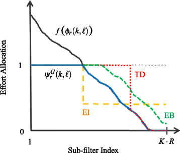

  

  Exemplary function f(ϕ _r (k,ℓ)) and corresponding $\psi ^{G}_{r}(k,\ell)$, plotted in sorted order of highest to lowest values, along with different criteria for modifying $\psi ^{G}_{r}(k,\ell)$ in case M _G(ℓ)<Q·K·R

  • Trickle Down (TD): When using this criterion (red), the surplus effort is redistributed via the trickle-down procedure, i.e., the sub-filters are filled up in sorted order of $\psi ^{G}_{r}(k,\ell)$. Allocating taps in this way respects the spectro-spatial sparsity present in the tap-inputs, but would most likely completely ignore sub-filters with the smallest magnitude tap-inputs.

  • Equal Income (EI): When using this criterion (orange), the same number of taps are allocated in all sub-filters for which $\psi ^{G}_{r}(k,\ell) < 1$. This has the beneficial effect that no sub-filters are ignored, but has the detrimental effect that the spectro-spatial sparsity present in the tap-inputs would most likely not be exploited for tap allocation.

  • Equal Bonus (EB): When using this criterion (green), the surplus effort is redistributed equally amongst all sub-filters for which $\psi ^{G}_{r}(k,\ell) < 1$. Allocating taps in this way respects the spectro-spatial sparsity present in the tap-inputs while making sure that all sub-filters get a few taps updated.

  Since the EB criterion attains a balance between exploiting spectro-spatial sparsity and not completely ignoring sub-filters, we decide to use this criteria in our proposed DEA scheme when M _G(ℓ)<Q·K·R, i.e.,

  $$ \psi^{D}_{r}(k,\ell) = \{1-\gamma(\ell)\} + \gamma(\ell) \cdot \psi^{G}_{r}(k,\ell), $$

  (31)

  where the superscript ^D denotes the proposed DEA scheme. The constant γ(ℓ) can be computed by substituting (31) into (22), yielding

  $$ \gamma(\ell) = \frac{K \cdot R - Q \cdot K \cdot R}{ K \cdot R - M_{\text{G}}(\ell)}. $$

  (32)

  Thus, each sub-filter has a minimum of ⌊{1−γ(ℓ)}·L⌋ taps selected in the ℓ ^th frame.

• Case 2: M _G(ℓ)>Q·K·R

  Similarly to Fig. 2, Fig. 3 shows an exemplary function f(ϕ _r (k,ℓ)) (black curve) and corresponding $\psi ^{G}_{r}(k,\ell)$ (blue curve) for the case M _G(ℓ)>Q·K·R. In order to satisfy the constraint, different criteria can be used for modifying $\psi ^{G}_{r}(k,\ell)$:

  Fig. 3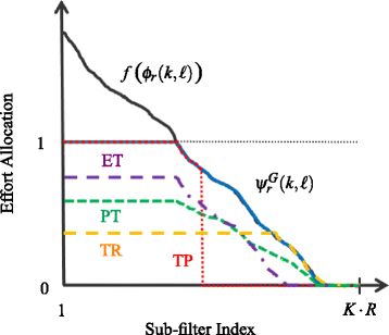

  

  Exemplary function f(ϕ _r (k,ℓ)) and corresponding $\psi ^{G}_{r}(k,\ell)$, plotted in sorted order of highest to lowest values, along with different criteria for modifying $\psi ^{G}_{r}(k,\ell)$ in case M _G(ℓ)>Q·K·R

  • Tax the Poor (TP): When using this criterion (red), the constraint is satisfied by decreasing the number of taps allocated to sub-filters with the lowest $\psi ^{G}_{r}(k,\ell)$. Such a scheme typically results in highly unequal tap allocation, with all taps reserved for a small number of sub-filters with the largest magnitude tap-inputs.

  • Tax the Rich (TR): When using this criterion (orange), the constraint is satisfied by decreasing the number of taps allocated to sub-filters with the highest $\psi ^{G}_{r}(k,\ell)$. This scheme has the beneficial effect that the majority of sub-filters are not ignored when allocating taps but has the detrimental effect that the spectro-spatial sparsity present in the tap-inputs is most likely not exploited for tap allocation.

  • Equal Tax (ET): When using this criterion (violet), the constraint is satisfied by decreasing the same number of taps from all K·R sub-filters. At first, this looks like a fair way of subtracting taps as it respects the spectro-spatial sparsity in the tap-inputs. However, it can be observed that this criterion ignores sub-filters with the smallest magnitude tap-inputs, as it takes away any small number of taps that may have been previously allocated to them.

  • Proportionate Tax (PT): When using this criterion (green curve), the constraint is satisfied by uniformly scaling down the number of allocated taps in the different sub-filters. Allocating taps in this way respects the spectro-spatial sparsity present in the tap-inputs, while ensuring that lesser number of taps are reduced from sub-filters with smaller $\psi ^{G}_{r}(k,\ell)$.

  Since the PT criterion attains a good balance between exploiting spectro-spatial sparsity and not completely ignoring sub-filters, we decide to use this criterion in our proposed DEA scheme when M _G(ℓ)>Q·K·R, i.e.,

  $$ \psi^{D}_{r}(k,\ell) = \delta(\ell) \cdot \psi^{G}_{r}(k,\ell), $$

  (33)

  where the constant δ(ℓ) can be computed by substituting (33) into (22), yielding

  $$ \delta(\ell) = \frac{Q \cdot K \cdot R} {M_{\text{G}}(\ell)}. $$

  (34)

The proposed DEA scheme can thus be summarized as

$$ {\begin{aligned} \psi^{D}_{r}(k,\ell) =\left\{ \begin{array}{ll} \{1-\gamma(\ell)\} + \gamma(\ell) \cdot \psi^{G}_{r}(k,\ell), & \text{if}~M_{\text{G}}(\ell) < Q \cdot K \cdot R \\ \delta(\ell) \cdot \psi^{G}_{r}(k,\ell), & \text{if}~ M_{\text{G}}(\ell) \geq Q \cdot K \cdot R. \end{array} \right. \end{aligned}} $$

(35)

The number of taps selected to be updated in the sub-filter $\underline {\hat {H}}_{r}(k,\ell)$ using the DEA scheme is finally determined by substituting (35) into (19).

4 Simulations, results and discussion

In this section, we present the reference signals and algorithmic parameters used, as well as the different metrics used to analyze signal sparsity, tap selection, and echo cancellation performance. We perform a sparsity analysis of the multichannel reference signals, individually across the three dimensions of subbands, channels, and filter length, as well as jointly across multiple dimensions. We then analyze the effect of using the different tap selection schemes on the echo cancellation performance obtained for the different types of reference signals used.

4.1 Signals and algorithmic parameters

In our simulations, we use time-domain reference signals at a sampling frequency of f _s =16 kHz. The different reference signals used can be divided into two categories:

• Synthetic signals

  • Mono brown and white noise signals, i.e., signals whose power densities change at the rate of -6 and 0 dB/octave, respectively.

  • Stereo white noise signal.

• Real-world signals

  • Mono speech signals (TIMIT database)

  • Surround-sound movie signals (Dolby Digital 5.0 format)

  • Surround-sound concert signals (Dolby Digital 5.0 format)

The acoustic impulse responses have been measured in a room with T ₆₀≈550 ms, with the microphone and the five loudspeakers placed on a circle of 3 m radius. The microphone was placed at a height of 1.2 m, the centre (C) loudspeaker was placed directly 0.85 m below the microphone, the front left (FL) and right (FR) loudspeakers were placed at the same height and 30 ^o either side of the microphone, and the side left (SL) and right (SR) loudspeakers were placed 0.4 m above and 110 ^o either side of the microphone, respectively. The acoustic echo signal d _r is obtained by convolving the reference signal x _r with the corresponding impulse response h _r for V _r =200 ms. We assume no near-end speech signal (s(n)=0) and no additive near-end noise signal (b(n)=0) for our simulations. For the mono reference signals, we use the impulse response corresponding to the C loudspeaker only, while for the stereo white noise signal, we use the impulse responses corresponding to the FL and FR channels. The time-domain signals have been transformed into the subband domain using STFT processing with N _FFT=512 (i.e., K=257) using a Hanning window and an overlap of 75%. We use a filter length L=20 for the MAEC filters, which corresponds to N _FFT·{1+0.25·(L−1)} samples or 184 ms. For updating the MAEC filters, a fixed step-size of μ=0.1 and regularization parameter of ε=10⁻⁶⁰ have been used.

4.2 Performance measures

Here, we present the different metrics used to analyze the sparsity present in the reference spectra, to analyze the performance of the different tap selection schemes in exploiting signal sparsity and to measure the echo cancellation performance.

4.2.1 Sparsity metric

To analyze the sparsity in the multichannel reference spectra across subbands, channels and frames, different metrics exist, such as the l ₀-norm, the l ₁ norm, the Gini index [31] and the Hoyer metric [32]. For an N-element (non-zero) vector $\underline {u} = [u_{0} \ldots u_{N-1}]$, where the elements are sorted in order of magnitude |u ₀|≤…≤|u _N−1|, the Gini index is defined as

$$ g(\underline{u}) = 1 - 2 \cdot \sum\limits_{j=0}^{N-1} \left(\frac{N-j-0.5}{N}\right) \cdot \frac{|u_{j}|}{\sum_{i=0}^{N-1} |u_{i}|}. $$

(36)

On the one hand, for the extreme case where |u ₀|=…=|u _N−1|, i.e., no sparsity in $\underline {u}$, $g(\underline {u}) = 0$. On the other hand, for the extreme case where |u ₀|=…=|u _N−2|=0 and |u _N−1|≠0, i.e., very high sparsity in $\underline {u}$, $g(\underline {u}) = 1 - \frac {1}{N}$, which for a large value of N is approximately equal to 1. Thus, the sparser the vector, the higher the Gini index.

Furthermore, the Gini index exhibits the following properties:

• Limited range: $0 \leq g(\underline {u}) \leq 1$.

• Scaling invariance: $g(a \cdot \underline {u}) = g(\underline {u})$, ∀$a \in \mathcal {R}$.

• Sensitivity to addition: $g(a + \underline {u}) < g(\underline {u})$, ∀$a \in \mathcal {R}, a > 0$.

• Cloning invariance: $g(\underline {u}) = g([\underline {u} \hspace {3pt} \underline {u}]) = g([\underline {u} \hspace {3pt} \underline {u} \hspace {3pt} \underline {u}])$

• Sensitivity to zero-padding: $g([\underline {u} \hspace {3pt} 0]) > g(\underline {u})$

The cloning invariance property allows a fair comparison of the sparsity of vectors with different number of elements. This is an important consideration, as we want to compare the sparsity of the reference spectra across the different dimensions of subbands, channels and frames. Note that the oft-used Hoyer metric does not exhibit this invariance and is hence not suited for comparing vectors with different number of elements.

4.2.2 Tap selection performance

In order to quantify the closeness of a tap selection scheme to full tap selection, we use the so-called Closeness Measure [19, 20] which is defined as the ratio of the energy of the M selected tap-inputs to the energy of all tap-inputs, i.e.,

$$ \xi \biggl(\underline{\alpha}(\ell), \underline{\mathbf{X}}(\ell) \biggr) = \frac{||\underline{\alpha}(\ell) \odot \underline{\mathbf{X}}(\ell)||_{2}^{2} } { ||\underline{\mathbf{X}}(\ell)||_{2}^{2} }. $$

(37)

For full filter update, i.e., $\underline {\alpha }(\ell) = \underline {1}$, we obviously obtain ξ=1. For a given Q, the 3DM scheme maximizes the Closeness Measure in every frame, as it selects the M largest magnitude tap-inputs. The expectation and assumption is that the tap selection scheme yielding the largest Closeness Measure also results in the smallest difference in AEC performance compared to updating the filters using full tap selection.

4.2.3 Echo cancellation performance

The echo cancellation performance is evaluated using the echo return loss enhancement (ERLE) [2], which is defined as

$$ \text{ERLE}(n) = 10 \cdot \log_{10} \frac{E \left[ d^{2}(n) \right] } { E \left[ \left(d(n) - \hat{d}(n) \right)^{2} \right] }, $$

(38)

where $\hat {d}(n)$ is the time-domain signal corresponding to the total MAEC filter output $\hat {D}(k,\ell)$ and E[·] denotes the statistical expectation operator. In practice, the ERLE is computed by approximating the expectation operator with the current sample value. The speed of convergence of the MAEC filters is assessed using the t ₂₀ metric, which is the time required for the ERLE to reach 20 dB.

4.3 Sparsity analysis

In this section, we present an example to illustrate the amount of sparsity typically present in real-world multichannel spectra across subbands, channels and frames, and also jointly across multiple dimensions. Figure 4 depicts the waveform of a 10 s segment from the soundtrack of a 5-channel movie signal, with the spectrograms of the C, FL, FR, SL and SR channels shown in the subplots below. Each magnitude spectrogram is composed of K=257 subbands and T=1247 frames. In this movie signal, the centre channel contains the speech content, while the surround-sound channels contain the background score.

Fig. 4

a Waveform of a 10-s segment from the soundtrack of a five-channel movie signal, with different channels distinguished by color; magnitude spectrogram of (b) centre (C), (c) front left (FL), (d) front right (FR), (e) side left (SL), and (f) side right (SR) channels, respectively

From these spectrograms, we first analyze the sparsity across subbands (spectral sparsity), across frames (temporal sparsity) and across channels (spatial sparsity). The Gini index for spectral sparsity in each channel is computed in every frame on a vector of K spectral coefficients, as exemplarily shown in Fig. 4 b for the centre channel using the magenta box in frame 200. Similarly, the Gini index for temporal sparsity in each channel is computed on a vector of T spectral coefficients in every subband, as shown using the blue box for subband 150. The Gini index for spatial sparsity in each subband and frame is computed on a vector of R spectral coefficients, as exemplarily shown using the black boxes for the first subband in frame 400. The Gini indices so obtained for spectral, temporal and spatial sparsity are shown in Fig. 5 a, b, and c, respectively. It can be observed that the multichannel reference spectra displays a fairly high amount of sparsity across all the three dimensions individually, with Gini indices on average above 0.5 (except for temporal sparsity in the surround-sound channels). The centre channel displays higher temporal sparsity as compared to the surround-sound channels as it contains time-varying speech content, while the surround-sound channels contain the background score, which varies slowly with time.

Fig. 5

Gini indices for a 10-s segment from the soundtrack of a five-channel movie signal; (a) spectral sparsity in each channel and joint spectro-spatial sparsity, (b) temporal sparsity in each channel and joint spatio-temporal sparsity, (c) spatial sparsity in each subband and frame, (d) joint spectro-temporal sparsity in each channel and joint spectro-spatio-temporal sparsity

Additionally, we analyze the sparsity present in the spectra jointly across multiple dimensions. In Fig. 5 a, the black curve displays the Gini index for the joint spectro-spatial sparsity, computed in every frame on a vector with K·R spectral coefficients. Similarly, in Fig. 5 b, the black curve displays the Gini index for the joint spatio-temporal sparsity, computed in every subband on a vector with R·T spectral coefficients. The Gini index for the joint spectro-temporal sparsity in each channel is computed by processing the magnitude spectrogram of that channel and is plotted in Fig. 5 d, along with the joint spectro-spatio-temporal sparsity for all K·R·T coefficients. From this figure, it can be clearly observed that the multichannel reference spectra exhibit even higher levels of sparsity when analyzed across multiple dimensions, with Gini indices on average above 0.85. This provides the motivation to exploit sparsity jointly across subbands, channels and frames for the purpose of tap selection.

Figure 6 shows the Gini indices for the joint spectro-spatio-temporal sparsity for the different considered reference signals. The stereo white noise signal is chosen to be spatially sparse, with an inter-channel broadband power ratio of 20 dB. Firstly, it can be observed for the synthetic signals that the spectrally colored brown noise signal and the stereo white noise signal are obviously more sparse than the mono white noise signal. Secondly, it can be observed that typical real-world signals such as mono speech and five-channel movie and concert signals also display high amounts of sparsity.

Fig. 6

Gini indices for joint spectro-spatio-temporal sparsity for different reference signals

4.4 Analysis of tap selection schemes for synthetic signals

In this section, we analyze the effect of using the constrained tap selection schemes from Section 3 (3DM, SPU, FEA and DEA) for synthetic signals.

4.4.1 Effect of Spectral Coloration

For the different tap selection schemes, Fig. 7 shows the number of taps selected in each subband when using a mono brown signal with Q=0.2. For the 3DM and SPU schemes, a larger number of taps are selected in the low-frequency subbands which contain the larger magnitude tap-inputs, while the high-frequency subbands with the smallest magnitude tap-inputs get no taps selected. Since the FEA scheme does not exploit spectral sparsity, it allocates an equal number of taps in all sub-filters irrespective of the signal content. The proposed DEA scheme achieves a balance by allocating more taps to sub-filters with larger magnitude tap-inputs (thereby exploiting spectral sparsity), while not completely ignoring the sub-filters with the smallest magnitude tap-inputs.

Fig. 7

Number of taps selected in each subband when using the 3DM, SPU, FEA and DEA tap selection schemes for a mono brown noise signal (Q=0.2)

4.4.2 Effect of Inter-Channel Power Ratio

We now consider a stereo white noise signal, where the broadband power of the first and the second channel is denoted as λ ₁ and λ ₂, respectively. Figure 8 shows the effect of the inter-channel power ratio $\frac {\lambda _{2}}{\lambda _{1}}$ on the number of taps selected in the sub-filters of the first channel (as a fraction of the M taps selected in both channels) for the different tap selection schemes with Q=0.2. When using the 3DM and SPU schemes, for λ ₁>λ ₂, the sub-filters in the first channel get the majority of the M taps selected. Thus, both schemes are highly spatially selective, as hardly any taps of the sub-filters in the less dominant reference channel are updated (e.g., for the SPU scheme when the inter-channel power ratio is larger than 5 dB and for the 3DM scheme when the inter-channel power difference ratio is larger than 10 dB). Since the FEA scheme does not exploit spatial sparsity, it allocates an equal number of taps to the sub-filters in the first and the second channel (i.e., $\frac {M}{2}$ taps each), irrespective of the inter-channel power ratio. The proposed DEA scheme achieves a balance by allocating more taps to the sub-filters in the dominant reference channel (thereby exploiting spatial sparsity), while not completely ignoring the channel with the smaller magnitude tap-inputs.

Fig. 8

Effect of the inter-channel power ratio of a stereo white noise signal on the number of taps allocated to the sub-filters in the first channel (as a fraction of M taps allocated to both channels) when using the 3DM, SPU, FEA, and DEA tap selection schemes (Q=0.2)

4.4.3 Closeness Measure

For different values of Q, Fig. 9 depicts the Closeness Measure ξ obtained when using the different tap selection schemes for mono brown, mono white and stereo white noise signals. For the stereo white noise signal, an inter-channel power ratio of 20 dB has been chosen. This figure shows how close the different tap selection schemes are to full tap selection in terms of the energy of the selected tap-inputs. By design, the 3DM scheme maximizes the Closeness Measure for a given Q, and hence yields the highest values for each signal. For a highly sparse signal such as the mono brown signal, a very high value for the Closeness Measure (≈1) is obtained for the 3DM scheme even when only 10% of the total filter taps are selected (i.e., Q=0.1). This means that just 10% of the tap-inputs contain almost the entire energy. For the least sparse mono white noise signal, low values of the Closeness Measure are obtained for all schemes, especially for the SPU scheme. For example, for Q=0.5, a Closeness Measure of about 0.85 is obtained for the 3DM, FEA and DEA schemes, whereas a Closeness Measure of about 0.6 is obtained for the SPU scheme. The Closeness Measure values obtained for the stereo white signal for all schemes lie in between those obtained for the more sparse mono brown noise signal and the less sparse mono white noise signal, except for the FEA scheme, which yields the same values as for the mono white noise signal. The SPU scheme gives high values for highly sparse signals and very low values for signals with low amounts of sparsity, while the proposed DEA scheme performs similarly to the 3DM scheme for highly sparse signals and similarly to the FEA scheme for signals with low amounts of sparsity.

Fig. 9

Closeness Measure as a function of Q for mono brown, mono white, and stereo white noise signals for different tap selection schemes

4.4.4 ERLE and t ₂₀

As shown by the previous experiments, depending on the spectral coloration and the inter-channel power ratio of the reference signals, each considered tap selection scheme results in a different distribution of the selected taps across subbands and channels, and a different Closeness Measure. Hence, it is to be expected that the tap selection schemes have an influence on the overall acoustic echo cancellation performance, i.e. ERLE and speed of filter convergence.

For mono brown, mono white and stereo white noise (inter-channel power ratio of 20 dB) signals, Fig. 10 a shows the ERLE convergence curves for the 3DM, SPU, FEA, and DEA tap selection schemes (Q=0.2), compared to full filter update (Q=1). Figure 10 b shows the corresponding t ₂₀ values for different values of the parameter Q. It can be observed that for signals with a high amount of spectral sparsity, such as the mono brown noise signal, the DEA scheme yields the best echo cancellation performance, while the 3DM and SPU schemes yield the poorest performance despite obtaining the highest values for the Closeness Measure. This is due to the highly spectrally selective nature of the 3DM and SPU schemes (discussed in Section 4.4.1), i.e., the sub-filters with the smallest magnitude tap-inputs do not have taps updated in every frame, resulting in very slow convergence of these sub-filters and thus negatively affecting the overall echo cancellation performance. For the least sparse mono white noise signal, it can be observed that the 3DM, FEA, and DEA schemes yield similar echo cancellation performance, while the SPU again yields the poorest performance. This may be due to the fact that the SPU scheme is the only one which completely ignores entire subbands when updating the filters, while the other schemes may allocate a few taps to each subband when the reference signal has a low amount of sparsity. For the spatially sparse stereo white noise signal, the DEA scheme performs better than the FEA scheme, both in terms of the converged ERLE value as well as the t ₂₀ values. For all considered signals, the ERLE and t ₂₀ values obtained by the proposed DEA scheme for Q=0.2 are very similar to those obtained for full filter update. Thus, the DEA scheme gives very similar echo cancellation performance to full filter update even when only 20% of the total MAEC filter taps are updated in every frame.

Fig. 10

(a) ERLE convergence curves for full filter update (Q=1) and for different tap selection schemes (Q=0.2), and (b) t ₂₀ values for different values of Q (for mono brown, mono white, and stereo white noise signals)

4.5 Analysis of tap selection schemes for real-world signals

Contrary to the synthetic (stationary) signals in the previous section, in this section we investigate the effect of using constrained tap selection schemes on the echo cancellation performance for (non-stationary) real-world signals.

For a mono speech signal, Fig. 11 shows the ERLE curves obtained when the MAEC filters are updated using the different tap selection schemes for Q=0.2 and for full filter update (Q=1) for a period of 10 s. For this signal, we find that even when only 20% of all filter taps are updated in every frame, both the 3DM scheme and the proposed DEA scheme typically perform as well as full filter update in terms of ERLE, with the FEA scheme performing slightly worse (about 1–2 dB). On the other hand, the SPU scheme performs significantly worse, yielding about 7–8 dB deterioration in terms of ERLE.

Fig. 11

(a) ERLE curves obtained for full update (Q=1) and for different tap selection schemes (Q=0.2) for a 10-s segment of a mono speech signal; (b) waveform of the 10-s segment of a mono speech signal

For a 5-channel concert signal, Fig. 12 shows the ERLE curves obtained when the MAEC filters are updated using the different tap selection schemes for Q=0.2 and for full filter update (Q=1) for a period of 30 s. For this signal, we find that even when only 20% of all filter taps are updated in every frame, both the 3DM scheme and the proposed DEA scheme perform almost identically to full filter update in terms of ERLE, with less than 1 dB deterioration, while the FEA scheme leads to about 2–4 dB deterioration in terms of ERLE. The SPU scheme again performs significantly worse, yielding about 10–12 dB deterioration in ERLE. It can be seen that around the 12-s mark, all schemes witness a sudden drop in ERLE. This is because the tap-input covariance matrix becomes ill-conditioned, leading to an increase in misalignment. However, it can also be observed that even though the FEA and DEA schemes have not been designed to tackle the misalignment problem, they do not deteriorate the problem further.

Fig. 12

(a) ERLE curves obtained for full update (Q=1) and for different tap selection schemes (Q=0.2) for a 30 -s segment of a 5-channel concert signal; (b) waveform of the 30 -s segment of a 5-channel concert signal

Additionally, Fig. 13 shows the number of taps $\mathcal {L}_{r}(k,\ell)$ updated in the different sub-filters in every frame using the DEA scheme for Q=0.2. It can be observed that the sub-filters in each channel get a small number of taps selected in every frame, where the number of taps updated across subbands depends on the spectral content present in each channel. As the centre channel for this signal consists of only speech, the tap allocation for the centre channel strongly resembles the spectrogram of a speech signal. As the surround-sound channels are mainly dominated by background score and low-frequency crowd noise but also contain some speech, this is reflected in how taps are allocated in the surround-sound channels.

Fig. 13

Number of taps $\mathcal {L}_{r}(k,\ell)$ updated in the different sub-filters in every frame for the (a) centre, (b) front left, (c) front right, (d) side left and (e) side right channels when using the DEA tap selection scheme for Q=0.2 for a 30-s segment of a 5-channel concert signal

5 Computational effort

When compared to full filter update, implementing a tap selection scheme requires some computational overhead, but still may result in significant savings when updating the MAEC filters, as only a fraction Q of the total N filter taps are updated in every frame. The computational effort per frame for implementing the different tap selection schemes and for updating the MAEC filters using the PUNLMS algorithm is given in Table 1. The computations have been divided into four categories, namely the number of additions (# Adds), multiplications (# Mults), divisions (# Divs) and comparisons (# Comps). Please note that all complex operations have been converted into an equivalent number of real operations, e.g. 1 complex multiplication has been counted as 4 real multiplications and 2 real additions.

Table 1 Computational effort

Figure 14 is an exemplary figure depicting the total computational effort required per frame for implementing tap selection and partial filter update for different values of Q. The numbers have been computed for K=257, R=5, and L=20 and by assuming that the comparison, multiplication and division operations are 1, 4 and 15 times as computationally expensive as an addition operation, respectively. The numbers have been plotted as a percentage of the computational effort required for full filter update, i.e., the effort required for updating the MAEC filters using the PUNLMS algorithm with Q=1. For these assumed settings, it can be observed that the total computational effort for the 3DM, SPU, FEA and DEA schemes is smaller than full filter update for Q<0.27, Q<0.95, Q<0.96 and Q<0.93, respectively. Hence, the SPU, FEA, and DEA schemes are almost always cheaper than full filter update. When only 20% of the MAEC filter taps are updated in every frame (Q=0.2), the 3DM scheme requires 94%, while the SPU, FEA, and DEA schemes require about 28% of the total computational effort required for full filter update. Using the SPU and DEA schemes results in slightly larger computational effort as compared to the FEA scheme due to the additional overhead required for computing η _r (k,ℓ) in (18) and $\psi ^{D}_{r}(k,\ell)$ in (35), respectively.

Fig. 14

Total computational effort required per frame for implementing the different tap selection schemes and for updating the MAEC filters using the PUNLMS algorithm as a function of Q. The numbers have been computed for K=257, R=5 and L=20 and have been plotted as a percentage of the effort required for full filter update

6 Conclusions

In this paper, different tap selection schemes for constrained partial updates of subband MAEC filters have been compared. Real-world multichannel signals have been analyzed and shown to be sparse across subbands (spectrally), channels (spatially), and frames (temporally). This sparsity is then exploited by different tap selection schemes for updating the MAEC filters. The MAEC system consists of a dedicated subband AEC filter for each loudspeaker channel, with each filter composed of multiple sub-filters, i.e., one sub-filter per subband per channel. The first tap selection scheme considered applied the well-known M-Max criterion on the multichannel input spectra across all three dimensions, and is hence called the 3DM scheme. This scheme jointly exploits the spectral, spatial and temporal sparsity in the input signals but typically results in some sub-filters having no taps updated. In order to avoid this problem, two new schemes have been presented which perform tap selection by applying the M-Max criterion only across filter length (and thereby exploit temporal sparsity for updating each sub-filter) and do not completely ignore the sub-filters with the smallest magnitude tap-inputs. The FEA scheme allocates a fixed number of taps to be updated in each sub-filter per frame, while the proposed DEA scheme exploits the joint spectro-spatial sparsity present in the input signals for dynamically allocating the number of taps to be updated in the different sub-filters. The new tap selection schemes have been compared to the state-of-the-art SPU tap selection scheme in the subband domain, which displays similar properties to the 3DM scheme. The proposed DEA scheme is designed such that it selects more taps in the sub-filters with larger magnitude tap-inputs (like the 3DM and SPU schemes) while not completely ignoring the sub-filters with smaller magnitude tap-inputs (like the FEA scheme). Simulation results for speech and music signals showed that in terms of ERLE and convergence speed, the 3DM and DEA schemes achieved almost identical echo cancellation performance compared to full filter update even when only 20% of the MAEC filter taps were updated in every frame, while the FEA and SPU schemes performed worse (about 2–4 dB and 10–12 dB deterioration in ERLE, respectively). The SPU, FEA and DEA tap selection schemes have a reduced computational cost compared to full filter update, while the 3DM scheme does not necessarily lead to reduction in computational complexity. Hence, in conclusion, the proposed DEA tap selection scheme yields almost identical echo cancellation performance compared to updating all filter taps at a significantly reduced computational cost.

7 Endnote

¹ It should be noted that the XM tap selection scheme [18–20] cannot be straightforwardly implemented in the subband domain and extended to more than two channels.

References

J Benesty, T Gansler, DR Morgan, MM Sondhi, SL Gay, Advances in Network and Acoustic Echo Cancellation (Springer-Verlag, Berlin, 2001).
E Hänsler, G Schmidt, Acoustic Echo and Noise Control - a Practical Approach (Wiley and Sons, Hoboken, NJ, 2004).
MM Sondhi, DR Morgan, JL Hall, Stereophonic acoustic echo cancellation—an overview of the fundamental problem. IEEE Sig. Process Lett. 2:, 148–151 (1995).
H Buchner, J Benesty, W Kellermann, in Adaptive signal processing: Application to real-world problems, ed. by J Benesty, Y Huang. Multichannel frequency-domain adaptive filtering with application to acoustic echo cancellation (Springer-VerlagBerlin/Heidelberg, 2003), pp. 95–128.
H Buchner, J Benesty, W Kellermann, Generalized multichannel frequency-domain adaptive filtering: efficient realization and application to hands-free speech communication. Signal Proc. 85(3), 549–570 (2005).
Y Huang, J Benesty, J Chen, Identification of acoustic MIMO systems: Challenges and opportunities. Signal Proc. 86(6), 1278–1295 (2006).
SC Douglas, Adaptive filters employing partial updates. IEEE Trans. Circ. Syst.-II Analog. Digit. Signal Proc. 44(3), 209–216 (1997).
T Schertler, Selective block update of NLMS type algorithms. Proc. IEEE Int. Conf. Acoust. Speech Signal Proc. Seattle USA.3:, 1717–1720 (1998).
T Aboulnasr, K Mayyas, Selective coefficient update of gradient-based adaptive algorithms. Proc. IEEE Int. Conf. Acoust. Speech Signal Proc. Munich Germany.3:, 1929–1932 (1997).
T Aboulnasr, K Mayyas, Complexity reduction of the NLMS algorithm via selective coefficient update. IEEE Trans. Signal Proc. 47(5), 1421–1424 (1999).
K Doǧançay, O Tanrikulu, Adaptive filtering algorithms with selective partial updates. IEEE Trans. Circ. Syst.-II Analog. Digit. Signal Proc.48(8), 762–769 (2001).
K Doǧançay, PA Naylor, Recent advances in partial update and sparse adaptive filters. Proc. Eur. Signal Proc. Conf. Antalya Turkey, 1–4 (2005).
PA Naylor, W Sherliker, A short-sort M-Max NLMS partial-update adaptive filter with application to echo cancellation. Proc. IEEE Int. Conf. Acoust. Speech Signal Proc. Hong Kong.5:, 373–376 (2003).
H Deng, M Doroslovački, New sparse adaptive algorithms using partial update. Proc. IEEE Int. Conf. Acoust. Speech Signal Proc. Montreal Canada.2:, 845–848 (2004).
J Benesty, DR Morgan, MM Sondhi, A better understanding and an improved solution to the specific problems of stereophonic acoustic echo cancellation. IEEE Trans. Speech Audio Proc. 6(2), 156–165 (1998).
AWH Khong, J Benesty, PA Naylor, Stereophonic acoustic echo cancellation: analysis of the misalignment in the frequency domain. IEEE Signal Proc. Lett. 13(1), 33–36 (2006).
M Ali, Stereophonic acoustic echo cancellation system using time-varying all-pass filtering for signal decorrelation. Proc. IEEE Int. Conf. Acoust. Speech Signal Proc. 6:, 3689–3692 (1998).
AWH Khong, PA Naylor, Reducing inter-channel coherence in stereophonic acoustic echo cancellation using partial update adaptive filters. Proc. Eur. Signal Proc. Conf. Vienna Austria.405–408 (2004).
AWH Khong, PA Naylor, A family of selective-tap algorithms for stereo acoustic echo cancellation. Proc. IEEE Int. Conf. Acoust. Speech Signal Proc. Philadelphia USA. 3:, 133–136 (2005).
AWH Khong, PA Naylor, Stereophonic acoustic echo cancellation employing selective-tap adaptive algorithms. IEEE Trans. Audio Speech Lang. Proc. 14(3), 785–796 (2006).
E Ferrara, Fast implementations of LMS adaptive filters. IEEE Trans. Acoust. Speech Signal Proc. 28:, 474–475 (1980).
JMP Borrallo, MG Otero, On the implementation of a partitioned block frequency domain adaptive filter (PBFDAF) for long acoustic echo cancellation. Signal Proc. 27:, 301–315 (1992).
JS Soo, K Pang, Multidelay block frequency domain adaptive filter. IEEE Trans. Acoust. Speech Signal Proc. 38(2), 373–376 (1990).
JJ Shynk, Frequency-domain and multirate adaptive filtering. IEEE Signal Proc. Mag. 9(1), 14–37 (1992).
S Haykin, Adaptive Filter Theory (Prentice Hall, Upper Saddle River, NJ, 1996).
X Lin, AWH Khong, M Doroslovački, PA Naylor, Frequency-domain adaptive algorithm for network echo cancellation in VoIP. EURASIP J. Audio Speech Music Proc.2008:, 1–9 (2008).
R Crochiere, A weighted overlap-add method of short-time Fourier analysis/synthesis. IEEE Trans. Acoust. Speech Signal Proc. 28:, 99–102 (1980).
DE Knuth, The Art of Computer Programming, vol. 3 (Addison-Wesley, Reading, MA, 1973).
I Pitas, Fast algorithms for running ordering and max/min calculation. IEEE Trans. Circ. Syst. 36(6), 795–804 (1989).
NK Desiraju, S Doclo, T Gerkmann, T Wolff, Efficient multi-channel acoustic echo cancellation using constrained sparse filter updates in the subband domain. Proc. ITG Symp. Speech Commun. Erlangen Germany.1–4 (2014).
NP Hurley, ST Rickard, Comparing measures of sparsity. IEEE Trans. Inform. Theory. 55(10), 4723–4741 (2009).
PO Hoyer, Non-negative matrix factorization with sparseness constraints. J Mach. Learn. Res. 5:, 1457–1469 (2004).
Acknowledgements
The research leading to these results has received funding from the European Union’s Seventh Framework Programme (FP7/2007-2013) project DREAMS under grant agreement ITN-GA-2012-316969. The authors would also like to acknowledge the contribution of Anirudha Kalya in helping develop the DEA tap selection scheme.
Author information
Authors and Affiliations
Contributions
The contribution of the first author consists of developing the main algorithmic idea, performing simulations, analyzing the simulation results and drafting the article. The contribution of the second and third authors consist of critically discussing the developed algorithms and the simulation results with the first author, and proofreading and revising the article. All authors read and approved the final manuscript.
Corresponding author
Ethics declarations
Competing interests
The authors declare that they have no competing interests.
Publisher’s Note
Springer Nature remains neutral with regard to jurisdictional claims in published maps and institutional affiliations.
Rights and permissions
Open Access This article is distributed under the terms of the Creative Commons Attribution 4.0 International License (http://creativecommons.org/licenses/by/4.0/), which permits unrestricted use, distribution, and reproduction in any medium, provided you give appropriate credit to the original author(s) and the source, provide a link to the Creative Commons license, and indicate if changes were made.
About this article
Cite this article
Desiraju, N., Doclo, S. & Wolff, T. Efficient multichannel acoustic echo cancellation using constrained tap selection schemes in the subband domain. EURASIP J. Adv. Signal Process. 2017, 63 (2017). https://doi.org/10.1186/s13634-017-0497-5
Received:
Accepted:
Published:
DOI: https://doi.org/10.1186/s13634-017-0497-5