Radon spectrogram-based approach for automatic IFs separation

Abstract

The separation of overlapping components is a well-known and difficult problem in multicomponent signals analysis and it is shared by applications dealing with radar, biosonar, seismic, and audio signals. In order to estimate the instantaneous frequencies of a multicomponent signal, it is necessary to disentangle signal modes in a proper domain. Unfortunately, if signal modes supports overlap both in time and frequency, separation is only possible through a parametric approach whenever the signal class is a priori fixed. In this work, time-frequency analysis and Radon transform are jointly used for the unsupervised separation of modes of a generic frequency modulated signal in noisy environment. The proposed method takes advantage of the ability of the Radon transform of a proper time-frequency distribution in separating overlapping modes. It consists of a blind segmentation of signal components in Radon domain by means of a near-to-optimal threshold operation. The inversion of the Radon transform on each detected region allows us to isolate the instantaneous frequency curves of each single mode in the time-frequency domain. Experimental results performed on constant amplitudes chirp signals confirm the effectiveness of the proposed method, opening the way for its extension to more complex frequency modulated signals.

1 Introduction

Frequency modulated (FM) signals appear everywhere in applications as they well model a large class of signals including radar, audio, seismic, biosonar, and gravitational waves [1–4]. In a real scenario, a FM signal is multicomponent, i.e., it consists of the superposition of oscillating components having specific time-dependent amplitudes and frequencies [5, 6]. Given a multicomponent signal (MCS), a fundamental goal in various applications is the recovery of its single modes (decomposition problem) which represents a difficult task if the modes interfere [4, 7–9].

In the literature, there exist several methods devoted to addressing this issue. Even though methods like Empirical Mode Decomposition (EMD) [10] extract signal oscillatory components (i.e. its intrinsic mode functions) directly in the time domain, most of the existing approaches are based on time-frequency (TF) signal analysis [11–13] as it provides an efficient characterization of non-stationary signals.

A good TF transform is designed to concentrate the energy of a monocomponent signal around the ridge curve or instantaneous frequency (IF)—defined as the time derivative of signal phase. The higher the energy concentration around ridge points, the better the TF transform. If MCS modes present non-overlapping TF supports, IF curves can be separated in TF domain by efficient methods such as reassignment, syncrosqueezing [14–16], S-Transform [17], whose main goal is actually to concentrate TF distribution around ridge points. Unfortunately, if IF curves are “too close” in TF domain, the separation task becomes harder. Neither EMD nor the above-mentioned TF methods offer a general solution to this problem, that still represents a very challenging goal in signal processing. That is why existing and more recent procedures are mostly signal-dependent. Indeed, they either assume a specific class for the phase/IF function or they consist of adaptive, parametric and local refinements of already existing approaches and/or transforms—a brief review of the state of the art methods is given in Section 2.

This paper aims at combining both strategies in a unique framework by further investigating and exploiting the concept of TF modes separability. The final goal is to develop a blind and automatic modes separation method. In particular, the work represents a step forward with respect to the preliminary study presented in [18], where authors proposed an energy-based signal modes separation method which combines TF analysis and Radon transform (RT), with limited assumptions on signals class. The main idea is that crossing modes in TF plane are mapped into distinct points in Radon domain. As a consequence, a thresholding operation is able to separate modes contribution in Radon domain and IF curves can be recovered by simply inverting RT on each separated component. As expected, the choice of threshold value is a delicate task, since part of the informative content may be removed, especially in the presence of noise. The aim of this paper is then: (i) to provide a method for the automatic selection of the separation threshold, (ii) to investigate the properties of TF transform that guarantees the enhancement of modes contribution in Radon domain, as well as their separability.

With regard to the first issue, the method in [19] has been considered, as it provides a computationally advantageous procedure for extracting useful information from noisy TF distributions, independently of the considered signal class. A minimum description length (MDL)-based criterion has been then proposed in order to automatically tune the parameters required by the threshold evaluation procedure in [19] when applied in the Radon domain.

With regard to the second point, the applicability conditions have been studied and tested on TF transforms having different properties, i.e., providing a more or less spread TF signal representation. In particular, the most interesting and quite counter-intuitive result is that TF transform is required to be enough spread around the ridge curve to map each signal mode into a separated, significant and connected component in the Radon domain.

The proposed approach is then twofold advantageous. On the one hand, it is completely automatic, adaptive, and robust to noise; on the other hand, it takes advantage of the limit, in terms of spread, of the TF transform to better emphasize the significant contribution of each signal mode in Radon domain.

Experimental results show that the use of short time Fourier transform (STFT) in TF analysis and the MDL criterion for the automatic tuning of threshold value allows us to properly separate signal modes while being robust to noise. The extension of the proposed method to other distributions is also investigated with particular reference to Radon-Wigner (RW) transform.

The remainder of the paper is the following. Section 2 briefly reviews the state of the art methods. Section 3 contains the main definitions and properties of the transforms used in the proposed method: Wigner-Ville distribution, short time Fourier transform and Radon transform. Section 4 presents a detailed description of the proposed modes separation method, while some numerical examples, results evaluation, and comparative studies are presented in Section 5. Finally, Section 6 draws the conclusions and future perspectives.

2 Brief state of the art

As mentioned in the Section 1, modes separation in overlapping MCSs is a hard and still open problem in signal processing. Despite the variety of proposed methods and mathematical tools, the complete separation of overlapping MCSs is reliable only for very specific cases. Approaches dealing with this issue can be divided in two categories: (i) methods assuming the signal class a priori and (ii) tracking peaks-based refinement techniques.

Concerning the first category, linear FM (LFM) signals can be separated by Radon transform (RT), chirplet transform [20], Radon-Wigner (RW) transform [21, 22] and Lv’s distribution [23], while sinusoidally modulated signals can be separated by using the inverse Radon transform [24]. Recently, new solutions have been proposed for multivariate MCSs, i.e., for those signals whose measurement is available from several channels [25]. In this framework, modes decomposition can be achieved also for very noisy signals via a sufficient number of sensors. More in general, de-chirping and filtering-based methods can be applied to the polynomial class as they consist of the removal of the “non-stationary term” of a chirp signal, so that a narrowband filter can be utilized to extract the target component. For instance, in [26], a discrete-time polynomial model for the signal phases is adopted in order to define a de-chirping method suitable for overlapping components; on the contrary, in [27] polynomial IF estimation is significantly improved in the non-separable case by selecting proper non-ridge points providing the same IF information.

With regard to the second category, several tracking peaks-based methods for IF estimation of overlapping components have been established. Most of them rely on a TF representation obtained by iteratively adapting the kernel to the signal under analysis, known as adaptive directional time-frequency distributions (ADTFDs). Maxima points extracted from ADTFD are the starting point for IF estimation. The latter is usually performed by some modifications of the Viterbi Algorithm, which is designed to find the optimal path through minimization of a proper penalty function. In order to avoid the so-called “switch problem,” that is the assignment of a ridge point to the wrong component, the penalty functions are defined to promote the local direction of the estimated ridge [28] as well as to impose the local monotonicity [29]. A similar peak-detection and tracking procedure promoting the direction of the estimated IF is proposed in [30]. In the above-mentioned methods, ridge path regrouping is achieved under the basic assumption that the set of detected peaks as a whole can reflect the global TF pattern of a MCS. Unfortunately, this hypothesis immediately fails to be satisfied if two modes interact in a destructive way. In this critical case, TFD can present much lower energy at the interference region and then the detected ridge curve can appear so deviated to not correlate at all with the global TF pattern. In order to overcome this problem, the works in [31–33] provide iterative procedures for enhancing spectrogram resolution, even in the non-separable and destructive case, by taking advantage of an evolution law for spectrogram. A different approach has been proposed in [34], where it has been proved that the energy of spectrogram of a MCS, computed with respect to the frequency variable, is still a time-varying MCS having fast decaying and predictable amplitude.

3 Methods

3.1 Wigner-Ville distribution and spectrogram

In this section, we recall TF tools and the main results behind the proposed work—for more details see [5].

The Wigner-Ville distribution (WVD) of a function $f\in L^{2}(\mathbb {R})$ in a TF point (u,ξ) is defined as

$$ {\rm{WV}}_{f}(u,\xi)=\int_{\mathbb{R}}f\left(u+\frac{\tau}{2}\right)f\left(u-\frac{\tau}{2}\right)e^{-i\tau\xi}\, d\tau\,. $$

(1)

WVD is a TF energy density obtained by the correlation between the signal f and its shifted copies. As a result, it presents high resolution properties which can be exploited to identify TF signal structure. Indeed, if f(t)=a(t) cosϕ(t) is a FM signal, WVD is well-concentrated on the ridge curve (u,ϕ^′(u)), also known as IF curve, and the following result holds

$$ \phi'(u)=\frac{\int_{\mathbb{R}}\xi \,WV_{f}(u,\xi)\,d\xi}{\int_{\mathbb{R}} WV_{f}(u,\xi)\, d\xi}. $$

(2)

Unfortunately, for a MCS f, i.e.,

$$ f(t) = \sum_{k=1}^{P} f_{k}(t) = \sum_{k=1}^{P} a_{k}(t) e^{i \phi_{k}(t)}, $$

(3)

where f_k is the kth mode having time-dependent amplitude a_k and phase ϕ_k and P is the number of components, the quadratic form of WVD leads to interference between modes (cross-terms), making ϕk′(t),k=1,…,P, detection more complicated. Even though cross-terms can be reduced by averaging WVD by means of proper kernels, it causes a loss of resolution that is undesirable in practical applications. On the other hand, the simultaneous cross-term suppression and preservation of energy concentration property is not a trivial task.

Spectrogram is the energy density corresponding to STFT. More precisely, given a function $f(t)\in L^{2}(\mathbb {R})$, its STFT at a TF point (u,ξ) is defined as

$$\begin{array}{*{20}l} S_{f}(u,\xi)=\int_{\mathbb{R}}f(t)g(t-u)e^{-i\xi t} \, dt \,, \end{array} $$

(4)

where g(t) is an even and real window. Hence, the spectrogram is defined as p(u,ξ)=|S_f(u,ξ)|².

It is worth noting that all TF distributions can be written as a WVD averaging; indeed spectrogram can be equivalently expressed as

$$ p(u,\xi)=\frac{1}{2\pi}\int_{\mathbb{R}}\int_{\mathbb{R}} WV_{f}(t,\omega)WV_{g}(t-u,\omega-\xi)dt\, d\omega\,. $$

(5)

As a result, spectrogram is a spreader distribution than WVD. Even though reassignment-like methods allow us to overcome this problem, their success is limited to separable components, i.e., f_k,f_j defined as in Eq. (3) and satisfying

$$ |\phi_{k}'(t) - \phi_{j}'(t)| \geq \Delta \omega,\,\, \forall\, t $$

(6)

where Δω is the frequency bandwidth of the analysis window—see Fig. 1. In fact, in case of signals having overlapping components, i.e., there exists $\bar {t}\in \Omega _{t}$ such that

$$ |\phi_{k}'(\bar{t}) - \phi_{j}'(\bar{t})|< \Delta \omega, $$

(7)

Fig. 1

Separable components. a Spectrogram. b Reassigned spectrogram. c WVD. d Ideal TF representation perfectly concentrated on IF curves

ridge curves resolution is quite limited in the non-separability region and then reassignment-like methods are not able to discriminate components, as depicted in Fig. 2. On the contrary, the joint use of TF analysis and RT allows us to reach this goal as a complementary separation condition property holds. In particular, the spread of the TF transform, which should be a limit, will actually represent a fundamental feature of the method proposed in this paper, as it will be explained in details in the sequel.

Fig. 2

Overlapping components. a Spectrogram. b Reassigned spectrogram. The non-separability region is emphasized by the dashed box. c WVD. d Ideal TF representation perfectly concentrated on IF curves

3.2 From TF to Radon domain

RT of a function $F(x,y)\in \mathbb {R}^{2}$ is defined as the integral along each straight line in $\mathbb {R}^{2}$. More precisely, the RT of F at a point $(r, \theta)\in \mathbb {R}^{2}$ is the projection of F along the direction identified by the parameters r and θ, i.e., [35]

$$ R_{F}(r,\theta)=\int_{\mathbb{R}} F(r\mathbf{n}_{\theta} + s\mathbf{n}_{\theta}^{\perp})\, ds, $$

(8)

where n_θ=(cosθ, sinθ) and $\mathbf {n}_{\theta }^{\perp }=(-\sin \theta, \cos \theta)$. A rotation of the coordinate system (x,y) by an angle θ gives the new coordinates

$$ \left[\begin{array}{l} x' \\y' \end{array}\right]= \left[\begin{array}{ll} \cos\theta & -\sin\theta \\ \sin\theta & \cos\theta \end{array}\right] \left[\begin{array}{l} x \\y \end{array}\right], $$

(9)

and RT can be rewritten as [35]

$$ R_{F}(r,\theta)=\int_{\mathbb{R}}F(r\cos\theta-s\sin\theta, r\sin\theta +s\cos\theta) ds\,. $$

(10)

RT is 2π-periodic with respect to θ; hence, the Fourier slice theorem allows for its inversion whenever all function projections with respect to θ∈[0,π) are known.

More precisely, F(x,y) can be then recovered by applying the backprojection formula

$$ F(x,y)=\frac{1}{\pi}\int_{0}^{\pi} R_{F}((x,y)\cdot\mathbf{n}_{\theta},\theta)\, d\theta\,. $$

(11)

Remark: In tomography, a filter-backprojection formula is adopted, since it is more suitable for removing the unwanted artifacts given by the inversion procedure and get a clear “target” image. Conversely to tomography, in this work the target to be reconstructed is spread all over the domain and the Gibbs effects are informative for our purpose; that is why the reduced formula in (11) is used.

As discussed in the sequel, the application of RT to spectrogram, referred as Radon spectrogram distribution (RSD), and to WVD maps non-separable modes in a domain where the separation task is feasible.

3.3 Resolution enhancement of overlapping components in Radon domain

RT of a TF distribution representing a LFM signal is well concentrated around the point (r₀,θ₀) uniquely identifying the ridge curve, which is a straight line in TF plane. In particular, RW peaks at (r₀,θ₀). That is why many approaches for LFM signals analysis rely on RW as well as some of its modifications. These latter, for instance Lv’s distribution [23], are designed to achieve high cross-term suppression and high resolution also for adjacent modes, i.e., parallel LFM in TF domain—an example is given in Fig. 3b.

Fig. 3

Representation in Radon domain by RSD and RW. a RT of the spectrogram in Fig. 1a. b RT of the WV transform in Fig. 1c. c RT of the spectrogram in Fig. 2a. d RT of the WVD in Fig. 2c

Non-linear FM MCSs have more spread representations in domain, and then detection task seems to be harder with respect to the linear case. Nevertheless, if signal modes do overlap in TF domain, a visual inspection of RT leads to an easy discrimination of each mode contribution, as shown in Fig. 3c, d. This observation has been exploited in [18] in order to disclose single modes, independently of the specific frequency modulation. More precisely, RT of spectrogram, i.e., RSD, is considered. Single modes in Radon domain were separated by simple thresholding, and the threshold level was chosen in order to promote sparsity. Then, maxima points on each detected region R_i was selected as a mode signature in Radon domain and the inverse RT has been applied only on those points. The center of mass (u,c_u), at each time u, of the resulting TF representation is the separated IF curve.

Unfortunately, as widely known, the choice of a proper threshold is a very delicate operation and a wrong setting may significantly affect the final result. Figure 4 depicts a non-linear chirp processed by the method proposed in [18], where a too large threshold value has been adopted. The final result is not acceptable since the quadratic IF behavior is almost completely lost (Fig. 4e). For a threshold value h∈[0, maxR], where R denotes RSD, l₀-norm is defined as the cardinality of the set {R≥h}, while the considered error is the pointwise absolute difference between the reconstructed curve (u,c_u) and the true IF curve (u,ϕ^′(u)) referred to a monocomponent signal. Figure 4f depicts the normalized l₀-norm and the corresponding normalized mean and maximum error in the reconstruction. In Fig. 4f, the threshold level is represented by a vertical dashed line; as it can be noticed, it corresponds to high concentration (normalized l₀-norm is close to 0) but also to large mean error. This suggests that a sufficient low threshold value should be considered in order to obtain an accurate result. It is worth observing that in the multicomponent framework, the interaction between modes in Radon domain should also be taken into account. Therefore, the threshold value should allow for a trade-off between accuracy and localization.

Fig. 4

Threshold operation and reconstruction. a Spectrogram of a quadratic chirp. b RSD. c Threshold RSD at level h = 180. d Signature. e Reconstructed IF curve. fl₀-norm and errors behavior. Threshold level h = 180 is indicated by a vertical line

Assuming an optimal threshold value is available, one would exploit high concentration properties of RW and process it in the same way as proposed in [18]. The problem in this approach is that a simple threshold operation on RW does not allow for direct components separation in Radon domain, which is necessary to achieve IF curves detection, see Fig. 5(d–f–h). In particular, it is required that the threshold operation provides a number of connected components equal to the number of signal modes, otherwise it will not be possible to achieve the desired decomposition by simply inverting RT, as depicted in Fig. 5(c–e–g). In addition, a trade-off between accuracy and localization is needed.

Fig. 5

Modes separation in Radon domain is necessary. a Spectrogram of a 3-components FM signal. b WVD. c RSD. d RW. e Threshold RSD. f Threshold RW. g Inverse RT of (e). h Inverse RT of (f). If components are not properly isolated in Radon domain, IRT does not allow signal modes separation in TF domain

For these reasons, in this work, we propose to adopt an advanced adaptive thresholding-based technique for the extraction of useful content in a TF distribution [19] directly in Radon domain; the aim is to still use method in [18] for single-modes separation. Unfortunately, the method proposed in [19], denoted by $\mathcal {M}$, is based on the assumption that components to be separated appear concentrated in continuous energy regions, making it not suitable for RW processing. That is why, in order to guarantee the continuity of modes energy, a more spread distribution, namely RSD, has been adopted in this paper. In other words, RT somehow compensates for the lower resolution of spectrogram. The sparsity of the representation is then reached by selecting only a subset of “good” points in Radon domain, as it will be clearer in the sequel.

4 Extraction of RSD informative content

As discussed in the previous section, overlapping components look discernible in Radon domain. The question now is how efficient component separation can be while preserving high anti-noise performance.

The following conditions are assumed:

• (i) The number of modes is known and it is significantly smaller than the length of the analyzed signal; moreover, signal components are scattered in Radon domain;

• (ii) Signal modes in Radon domain are concentrated around a curve (IF signature), and they consist of continuous energy regions which emerge from the basically flat noisy background.

It is worth observing that the assumption on the number of components can be relaxed by adopting a counting procedure, for instance, the one proposed in [36], which is based on the analysis of the short-term Rényi entropy and allows for estimating the local number of components, even in the overlapping case.

Furthermore, additional conditions are assumed for RSD of overlapping modes:

• Signal modes in Radon domain have comparable amplitudes;

• For each mode, IF signature is a subset of useful information and it is disjointed from regions related to the other modes.

In this scenario, a proper amplitude threshold operation provides a segmentation of the single components composing the signal.

The novel idea in this paper is then to adopt method $\mathcal {M}$ proposed in [19] to obtain a near-to-optimal thresholding operation which is able to both extract useful information from Radon spectrogram distribution and achieve a signal segmentation, exploiting Radon capability of enhancing overlapping modes resolution.

It is worth observing that assumptions (i) and (ii) make method $\mathcal {M}$ suitable for RSD analysis. In addition, since $\mathcal {M}$ depends on the setting of some parameters, their automatic tuning is proposed by taking advantage of the minimum description length (MDL) strategy.

4.1 Extraction of useful information by adaptive thresholding

This section briefly reviews method $\mathcal {M}$ [19]. It consists of two main steps: the first one automatically partitions the observed distribution into K classes through K-means algorithm; the second one distinguishes between classes corresponding to noise and useful coefficients by applying the ICI rule. The final output is the distribution defined as the union of classes detected as useful information.

Given a set of observations C=ρ(n,m),n=1,…,N,m=1,…,M and set $K\in \mathbb {N}$, K-means algorithm provides a partition {C_k}_k=1,…,K of C by minimizing the within-cluster sum of squares, i.e.,

$$ \arg\min_{C} \sum_{k=1}^{K}\sum_{\rho(n,m)\in C_{k}} ||\rho(n,m)-\mu_{k}||^{2} $$

(12)

where μ_k is the mean of subset C_k. As a result, the analyzed distribution ρ is partitioned into K classes by setting

$$ \rho_{k}(n,m) =\left\{\begin{array}{l} \rho(n,m), \quad \text{if }\rho(n,m)\in C_{k}\\ \quad 0,\quad \quad \text{otherwise.} \end{array}\right. $$

(13)

At this point, the partition {ρ_k}_k=1,…,K itself gives no information concerning the informative classes. Based on condition (ii), noisy classes are identified as the ones having significantly larger supports with respect to useful classes, which conversely are assumed to be concentrated. Assuming that, for each k, coefficients belonging to one class ρ_k present equal amplitudes, the energy E(k) of the kth amplitude normalized class is defined as the l₀-norm of the class and processed in order to distinguish between noisy and informative classes, i.e., further partitioning C={C_noise,C_I}, with

$$\begin{array}{@{}rcl@{}} C_{{\rm{noise}}}&=&\{ C_{k} | k=1,..,k^{+} \}\\ & \text{and } C_{I}=&\{ C_{k} | k=k^{+}+1,..,K \}. \end{array} $$

(14)

Method $\mathcal {M}$ determines the separation index k⁺ which identifies the class with the largest index containing mainly noise, by tracking the intersection of confidence intervals of E(k) (ICI rule) and identifies the classes ρ_k for k⁺<k≤K as the extracted useful information.

Denoting by $\tilde {E}(k)$, the ideal energy, i.e., the one corresponding to $\tilde {C}_{I}$ which only contains useful information and by $\hat {E}(k,i)$ its estimate calculated as a weighted average of i(k) energies E(k), the pointwise mean squared error (MSE) of $\hat {E}(k,i)$ is

$$ {\rm{MSE}}(k,i)=\sigma^{2}(k,i) +\omega^{2}(k,i), $$

(15)

where σ²(k,i) is the estimation variance and ω²(k,i) is the estimation bias and MSE minimal value, for each k, is achieved by selecting the index i^∗ providing the best trade-off between estimation variance and bias, i.e.,

$$ i^{*}(k)=\arg\min_{i(k)} MSE(k,i). $$

(16)

ICI rule is used to get an approximation of the optimal index i^∗, as explained below.

It can be proved that $\tilde {E}$ belongs to the confidence interval

$$ {\begin{aligned} D(k,i)=[L(k,i),U(k,i)]&=\left[\hat{E}(k,i)-\Gamma\sigma(k,i),\hat{E}(k,i)\right. \\& \left. +\Gamma\sigma(k,i){\vphantom{\hat{E}(k,i)-\Gamma\sigma(k,i)}}\right] \end{aligned}} $$

(17)

with probability 1−α,α∈[0,1] and Γ depends on the ratio of the upper-bound bias to the standard deviation of the ideal i^∗(k) and α. Based on this result, for each E(k), the ICI rule calculates the confidence intervals for a growing class of indices i(k)=1,2,…,K−k+1 and selects the larger index i⁺(k) such that the intersection is non empty, i.e.,

$$ i^{+}(k)=\arg\max_{i(k)} \{ \cap_{i(k)=1}^{K-k+1} D(k,i) \neq\emptyset\}, $$

(18)

as an approximation of the index i^∗(k).

ICI criterion can be rephrased in terms of L(k,i) and U(k,i) defined in Eq. (17), by defining the smallest upper and largest lower confidence limits calculated as

$$\begin{array}{*{20}l} \underline{U}(k,i)=min\{U_{j},\, j=1,\ldots,i\}, \end{array} $$

(19)

$$\begin{array}{*{20}l} \bar{L}(k,i)=max\{L_{j},\, j=1,\ldots,i\}, \end{array} $$

(20)

then the index i⁺(k) is the largest index satisfying $\bar {L}(k,i)\leq \underline {U}(k,i)$.

In order to reduce the computational cost, the first class ρ₁(n,m) is used as a reference noise structure to distinguish between noise and useful information. This choice is justified by assumptions (i) and (ii), and it preserves the quality of ICI algorithm performance. Therefore, k⁺=i⁺(1),C_I={C_k | i(1)>k⁺} and the extracted useful information is given by the sum

$$ \rho_{I}(n,m)= \sum_{k=k^{+}+1}^{K} \rho_{k}(n,m). $$

(21)

In this work, we set ρ(n,m)=R_P(r,θ).

It is worth observing that $\mathcal {M}$ depends on two parameters, i.e., the number of classes K and Γ, whose optimal values are not known in advance. The only prior information is about the number of components, which is assumed, as in the majority of similar methods.

We propose to select K and Γ as the ones providing the more concentrated useful information by means of MDL. Formally, a two-dimensional minimization of a proper MDL functional is performed, with the constraint on the number of signal components.

4.2 Automatic threshold tuning

Adaptive thresholding method $\mathcal {M}$ requires input parameters Γ and K, whose values can be automatically determined by means of MDL principle [37].

MDL principle is a formalization of Occam’s razor, and its application can provide a solution to the problem of model selection, i.e., the choice of the best explanation of data given limited observations. MDL principle states that the best model (hypothesis) describing a given set of data is the one that compresses data the most.

In this context, model selection is turned into best coding of data and the theoretical concept of explanation of data is turned into its length expressed in bits.

More precisely, given $\mathcal {H}=\{H_{1}, H_{2}, \ldots, H_{J}\}$ a list of candidate models to describe a set of data D, the best model $H\in \mathcal {H}$ explaining D is the one which achieves

$$ \min_{H\in\mathcal{H}}\left(L(H) +L(D|H) \right), $$

(22)

where L(H) is the length, in bits, of the description of the model H and L(D|H) is the length, in bits, of the description of data when encoded by model H [37].

It is worth pointing out that the word model refers to a set of probability distributions or functions sharing the same functional form—e.g., the “model of kth degree polynomials.” Conversely, a point model (point hypothesis, in general) is an instantiated model, i.e., a particular parameter setting for the considered model [37].

The adopted approach in this work is an instance of MDL, where the considered data D is RSD, a model for D is one of the possible distributions given by the adaptive thresholding algorithm $\mathcal {M}$ and the description of data is intended as the l₀-norm of the distribution.

According to the above notation, we use MDL to determine the best point model for RSD, i.e., the values of input parameters Γ and K yielding the best description of RSD through thresholding operation performed by $\mathcal {M}$. Thus, by denoting the model as H=(K,Γ), the functional to be minimized is

$$ \min_{(K,\Gamma)\in\mathcal{H}} \left(L((K,\Gamma)) +L(RSD|(K,\Gamma)) \right). $$

(23)

In practice, by fixing a range for parameters Γ and K, a 2D minimization on l₀-norm of the extracted distribution is performed, constrained to the number of modes, i.e., only parameter values giving a distribution such that number of connected components is equal to the number of signal modes are considered.

4.3 Proposed signal modes separation

Given f(t) as defined in (3), the proposed method first computes spectrogram p and the corresponding RSD R_p(r,θ), for all θ∈[0,π). Method $\mathcal {M}$ is applied to R_p(r,θ) with (K,Γ)∈Ω={K₁,…,K_l}×{Γ₁,…,Γ_q}. The parameters $(\bar {K}, \bar {\Gamma })$ realizing the minimum of Eq. (23) are chosen as the best explanation of RSD R_p(r,θ), by means of MDL principle. The application of method $\mathcal {M}$ instantiated by $(\bar {K}, \bar {\Gamma })$, i.e., $\mathcal {M}((\bar {K}, \bar {\Gamma }))$, corresponds to performing a near-to-optimal threshold operation on RSD R_p(r,θ) at level h. The output represents the extracted useful information, denoted by R_I, and it is partitioned in connected components R_i, i=1,…,P, corresponding to original signal modes. Each connected component is processed separately by taking the maxima points along the vertical direction. As a result, a signature of each signal mode in Radon domain is obtained. The inversion of RT on those points gives P TF representations IR_i that need to be refocused in order to obtain a good IF curve approximation. IR_i are post-processed by selecting the local centers of mass along the frequencies, providing IF curves separation, even in non-separability regions.

The whole proposed procedure is illustrated by the flow-chart in Fig. 6, and it can be summarized as follows: Step 1. Compute the spectrogram p of the input signal fStep 2. Compute RT of the spectrogram, i.e., RSD R_pStep 3. Apply method $\mathcal {M}$ to R_p with parameters (K,Γ)∈Ω={K₁,…,K_l}×{Γ₁,…,Γ_q} and compute l₀-norm of the output distributions $\mathcal {M}(K, \Gamma)$Step 4. Select $(\bar {K}, \bar {\Gamma })$ s.t. the MDL functional in eq. (23) is minimum and set $R_{I}=\mathcal {M}(\bar {K}, \bar {\Gamma })$Step 5. Determine the connected components R_i,i=1,…,P of distribution R_IStep 6. For each R_i

• 6.1 Extract the signature, i.e., for each θ, set r_θ= arg maxr(R_i(r,θ)) and set R_i(r,θ)=0 ∀ r≠r_θ

  Fig. 6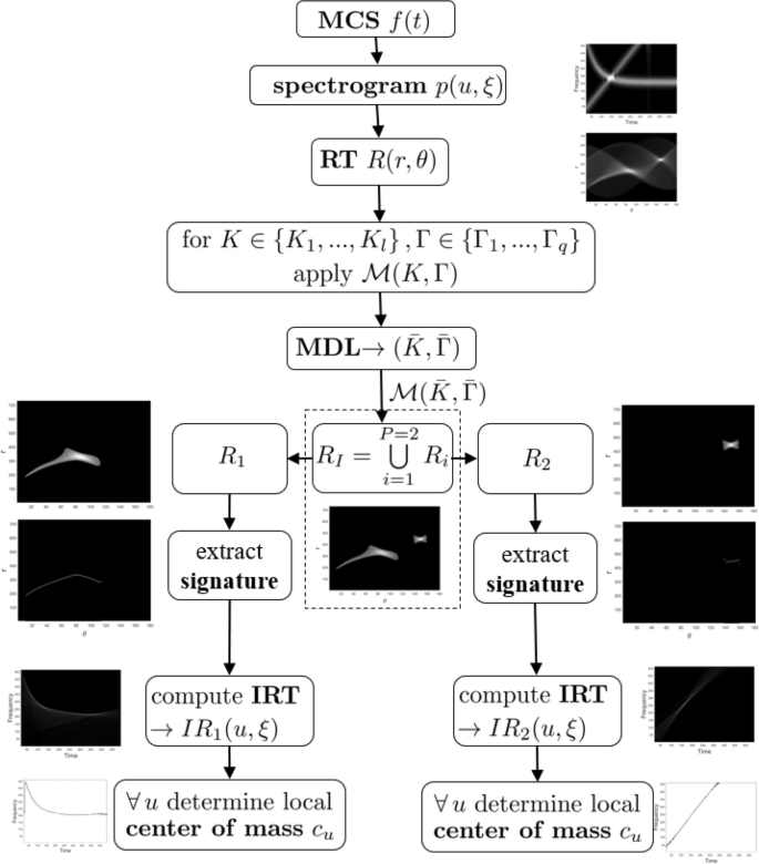

  

  Proposed signal modes separation flow-chart. A two-component signal is considered as illustrative example

• 6.2 Compute IR_i(u,ξ) as the inverse RT of R_i according to (11)

• 6.3 For each u, select ξ_u= arg maxξ(IR_i(u,ξ)) and the center of mass c_u around ξ_u

• 6.4 The curve (u,c_u), for all considered u, is the separated IF curve corresponding to the ith mode.

5 Results and discussion

The proposed modes separation method has been tested on several MCS having different frequency modulation. This section presents the most significant results concerning linear combination of the following polynomial and hyperbolic chirps of length L=512:

$$\begin{array}{*{20}l} f_{1}(t)&=\cos\left(\frac{L\pi}{4}t^{4}+ 0.2Lt\right)\\ f_{2}(t)&=\cos\left((0.38L\pi-100) t^{2} - 0.76 L \pi t+ 0.38 L \pi\right)\\ f_{3}(t)&=\cos\left(0.58 L\pi t\right)\\ f_{4}(t)&=\cos\left(\frac{4.5\pi}{0.7-t}+0.5Lt\right)\\ f_{5}(t)&= \cos\left(\frac{L\pi}{3}(1-t)^{2}\right) \\ f_{6}(t)&= \cos\left(0.6L\pi(t-0.5)^{3} +250t\right) \\ f_{7}(t)&= \cos\left(\frac{0.7L\pi}{2}(1 - t)\right)\ \end{array} $$

(24)

with $t\in \{\frac {1}{L},\frac {2}{L}, \ldots,1 \}$.

Signals are embedded in AWGN with different SNR levels. STFT is computed with a gaussian window of length s=44 and standard deviation $\sigma =\frac {s-1}{5}\approx 8.6$. MATLAB code implementing method $\mathcal {M}$ proposed in [19] has been downloaded from [38]. For each test signal, $\mathcal {M}$ is applied to RSD with parameter (K,Γ) varying in Ω = {3P,…16}×{0.20+i 0.05,i = 0,…,10}, where P denotes the number of signal modes. Range for parameter Γ is contained in the interval [0.20,0.70], since the value 0.5 has experimentally provided better results.

l₀-norm is computed for each iteration of $\mathcal {M}$, which provides exactly P connected components, and the parameters $(\bar {K}, \bar {\Gamma })\in \Omega$ achieving MDL functional minimum are selected as the best explanation of RSD.

Figure 7 refers to the three-component signal f(t)=1.5·f₁(t)+f₂(t)+1.1·f₃(t) embedded in AWGN (SNR= 9 dB). In this case, MDL functional minimum value is reached at $(\bar {K}, \bar {\Gamma })=(11,0.7)$. In order to visually prove the goodness of the corresponding threshold h, in Fig. 8, the representations in TF and Radon domain of the noise-free single components f₁,f₂,andf₃ are considered. Figure 8c depicts the behavior of l₀-norm and reconstruction errors regarding the single RSDs in Fig. 8b, while the threshold value increases. The vertical dashed lines indicate the threshold h corresponding to $(\bar {K},\bar {\Gamma })=(11,0.7)$. As it can be observed, in the non-linear case (top), h achieves a good trade-off between accuracy (mean error is moderate) and localization (l₀-norm value is low). Fig.7c–o shows the extracted classes by method $\mathcal {M}$ with parameters $(\bar {K},\bar {\Gamma })=(11,0.7)$ applied to RSD in Fig. 7b. Finally, Fig. 7p is the output distribution of $\mathcal {M}$, whose processing is shown in Fig. 9. Specifically, distribution in Fig. 7p is partitioned into connected components, which are depicted in Fig. 9a. The latter are processed by taking, for each θ, the maximum along the radial direction, which results in the signatures shown in Fig. 9b. Inverse RT of each signature is computed resulting in a blurred TF representation (see Fig. 9c) whose local center of mass approximates IF curve. Indeed, Fig. 9d shows three separated curves reflecting true IF behavior. Figure 10 shows the curve of average MSE values for SNR levels ranging from 0 to 16 dB.

Fig. 7

Detected classes and extracted useful information by method $\mathcal {M}$. a Noisy spectrogram of signal f(t)=f₁(t)+f₂(t)+f₃(t) in reference to Eq. (24). b RSD (contours). c–o classes extracted by method $\mathcal {M}$. p Extracted useful information R_I. Parameters given by MDL functional minimization are Γ=0.7,K = 11

Fig. 8

Noise-free components and reconstruction errors. Noise-free signals f₁,f₂, and f₃ defined in Eq. (24). a Spectrogram. b RSD. c Normalized l₀-norm and reconstruction errors versus the threshold value. The threshold value h given by $\mathcal {M}$ is indicated by a vertical line

Fig. 9

Result 1. a Connected components extracted by R_I in Fig. 7p. b Signatures. c IRT on signatures. d Separated IF curves

Fig. 10

Average MSE against SNR for signal f(t)=f₁(t)+f₂(t)+f₃(t)

The second experimental result concerns the two-component signal z(t) = 0.5·f₄(t)+0.5·f₅(t). AWGN at SNR = 12 dB has been added to the signal. MDL functional minimization provides parameters $(\bar {K},\bar {\Gamma })~=~(6,0.65)$. As shown in Fig. 11b, method $\mathcal {M}$ provides a threshold which is able to capture the linear chirp in Radon domain and also the spread distribution corresponding to the hyperbolic chirp. The proposed procedure is able to separate signal components, as illustrated in Fig. 11e, except for some errors at TF boundaries. The curve of average MSE values for SNR levels ranging from 0 to 16 dB is shown in Fig. 12.

Fig. 11

Result 2. a Spectrogram of the signal z(t)=f₄(t)+f₅(t) embedded in AWGN (left) and RSD (right). b Connected components obtained by applying method $\mathcal {M}$ with parameters K = 6,Γ = 0.65. c Signatures. d IRT on signatures. e Separated IF curves

Fig. 12

Average MSE against SNR for signal z(t)=f₄(t)+f₅(t)

Finally, Fig. 13 presents the result for the two-component signal w(t)=2·f₅(t)+f₇(t), embedded in AWGN at SNR= 14 dB. In this example, modes have multiple crossing points in TF domain as depicted by spectrogram in Fig. 13a (left). This results in a more confusing RSD Fig. 13a (right). MDL functional minimization gives $(\bar {K},\bar {\Gamma })=(6,0.6)$ and method $\mathcal {M}$ still provides a good representation, having two connected components. The latter is processed by the proposed method which gives two separated IF curves, as depicted in Fig. 13e. Figure 14 provides the average MSE curve against SNR.

Fig. 13

Result 3. a Spectrogram of the signal w(t)=f₆(t)+f₇(t) embedded in AWGN (left) and RSD (right). b Connected components obtained by applying method $\mathcal {M}$ with parameters K = 6,Γ = 0.6. c Signatures. d IRT on signatures. e Separated IF curves

Fig. 14

Average MSE against SNR for signal w(t)=f₆(t)+f₇(t)

5.1 Comparative studies

In order to compare the proposed procedure with some of the state of the art methods, we considered the signal

$$ v(t)=e^{i2\pi(21t^{3})} + e^{i2\pi(45t-15t^{3})} +e^{i2\pi(62t-15t^{3})}, $$

(25)

composed of two parallel non-LFM components intersecting with a non-LFM mode. The sampling rate is 256 Hz and the signal duration is 1 s. We compared our result with the one obtained by the modified Viterbi-ADTFD method [28], which combines adaptive TF analysis and a modified version of Viterbi algorithm. Spectrogram is shown in Fig. 15a while Fig. 15b, c, respectively, depict RSD and the detected components. Figure15d provides the result obtained by the proposed method, and Fig. 15e shows the average MSE against SNR for the two methods, with SNR levels ranging from 0 to 10 dB. As it can been observed, the two methods have quite comparable performance for higher SNR levels. However, it is worth observing that the proposed method is less precise in modes reconstruction at TF boundaries—see next subsection for details. To quantify this sensitiveness, the same figure shows MSE results provided by the proposed method when boundary points are omitted in the evaluation of the metric (star markers).

Fig. 15

Performance comparison. a Spectrogram of the signal v(t) in Eq. (25) embedded in AWGN at SNR level equal to 10 dB. b RSD. c Connected components detected by method $\mathcal {M}$ with parameters K = 11 and Γ = 0.65. d Result given by the proposed method. e Plot of average MSE against SNR for signal v(t). The proposed method and the modified Viterbi-ADTFD method in [28] are compared

It is also worth pointing out that, as the majority of tracking peak-based methods, the procedure introduced in [28] is based on a local estimate of IF that is used to adapt the kernel of the TFD. Furthermore, Modified Viterbi-ADTFD method is a searching technique and its performance strongly depends on the predefined set of candidate parameters. On the contrary, the proposed method works globally on the whole distribution, since RT is blindly computed on the spectrogram. Instead of adapting the transform to the analyzed signal, we map it into a domain where the information concerning IF is available and compact.

5.2 Some remarks

Reconstructed IF curves presented in the experimental results show some instabilities, especially at TF boundaries. This phenomenon is explained by the fact that slopes corresponding to points at TF boundaries are less represented in the compactly supported spectrogram domain, in the sense that the energy captured by RT is lower than the one observed in the whole plane $\mathbb {R}^{2}$. As a consequence, amplitudes regarding TF boundaries slopes are penalized in Radon domain. Furthermore, it is well-known that a single point in Radon domain is sufficient to recover a LFM signal, while the adopted threshold operation provides a more spread signature, which also results in a loss of accuracy. It turns out that an in-depth study aimed at defining a more efficient thresholding operation is needed. This should reasonably improve method performance at TF boundaries, making it more efficient also in high noise environment. The definition of a more advanced thresholding technique requires a further investigation of the mathematical structure of RSD, which is one of the main plan in our future research. As a result, condition (iii) on comparable amplitudes could be removed by integrating the proposed method with some iterative techniques, such as matching pursuit [5]. The strongest component should be extracted first and then the procedure should be iterated on the residual distribution till all the modes are recovered. The assumption on the number of components could be also removed by adopting a residual energy-based stopping criterion. This approach could reasonably allows for the applicability of the proposed method to real-life signals, which commonly present varying amplitudes, and it will be investigated in our future work.

Even though crossing modes represent a critical issue in modes separation problem in TF plane, it is not a necessary condition to be verified for the applicability of the proposed method. Nevertheless, two close and not intersecting components could be recognized as a unique contribution in the Radon domain. This is the case of close parallel components, as depicted in Fig. 3a, that can be solved by taking advantage of the knowledge of the number of modes: if just one contribution is detected in Radon domain, then the signatures can be obtained by extracting more than one local maximum for each θ. The analysis of modes having overlapping supports in Radon domain will be studied in-depth in our future work instead.

6 Conclusions

This paper has presented a novel strategy for the separation of overlapping IF curves referred to a MCS. In particular, the main contribution of the work has been the definition of the conditions under which the joint use of TF analysis and RT enables modes separation in non-linearly FM MCS. It relies on the key idea that RT maps non-separable modes in TF domain into a new domain where modes are distinguishable. An adaptive and automatic thresholding method for the extraction of informative content from the noisy RSD is adopted. The latter is also exploited to obtain a partition whose connected components are processed one by one in order to separate and recover each single IF curve.

The second main contribution of the work has been the observation that a spread TF transform allows for higher energy enhancement of signal modes in Radon domain, guaranteeing their easier separation by thresholding. On the contrary, too concentrated TF transforms result not useful for our purposes.

Experimental results performed on constant amplitude multicomponent FM signals confirm the efficiency of the proposed method in discriminating signal IF curves. The observation that crossing IF curves in TF domain are mapped into separated signatures in Radon domain opens the way to novel proposals for FM MCS analysis.

As future perspectives, we would like to study cases where some conditions are relaxed, as the one requiring comparable modes energy in Radon domain, and to quantify separability in Radon domain. The applicability to a TFD different from the spectrogram, with higher resolution, will be a focus of our future work. Reconstructed IF curves’ instabilities at TF boundaries and applicability to real-life signals will be also investigated.

References

P. Flandrin, in Wavelet Applications VIII, vol. 4391, ed. by H. H. Szu, D. L. Donoho, A. W. Lohmann, W. J. Campbell, and J. R. Buss. Time frequency and chirps (SPIE, 2001), pp. 161–175. https://doi.org/10.1117/12.421196.
B. Lyonnet, C. Ioana, M. G. Amin, in 2010 IEEE Radar Conference. Human gait classification using microdoppler time-frequency signal representations (IEEE, 2010), pp. 915–919. https://doi.org/10.1109/radar.2010.5494489.
T. Sakamoto, T. Sato, P. J. Aubry, A. G. Yarovoy, Texture-based automatic separation of echoes from distributed moving targets in uwb radar signals. IEEE Trans. Geosci. Remote Sens.53(1), 352–361 (2014).
H. Lee, T. H. Kim, J. W. Choi, S. Choi, in 2015 IEEE Conference on Computer Communications (INFOCOM). Chirp signal-based aerial acoustic communication for smart devices, (2015), pp. 2407–2415. https://doi.org/10.1109/infocom.2015.7218629.
S. Mallat, A Wavelet Tour of Signal Processing (Elsevier, 1999). https://doi.org/10.1016/b978-0-12-466606-1.x5000-4.
B. Boashash, Time-Frequency Signal Analysis and Processing: A Comprehensive Reference, (2015). https://doi.org/10.1016/c2012-0-00024-5.
B. Boashash, Estimating and interpreting the instantaneous frequency of a signal—part 2: Algorithms and applications. Proc. IEEE. 80(4), 540–568 (1992).
D. L. Stevens, S. A. Schuckers, Detection and parameter extraction of low probability of intercept radar signals using the hough transform. Global J. Res. Eng.15(6), 9–25 (2016).
D. -H. Pham, S. Meignen, High-order synchrosqueezing transform for multicomponent signals analysis with an application to gravitational-wave signal. IEEE Trans. Sig. Process.65(12), 3168–3178 (2017).
N. E. Huang, Z. Shen, S. R. Long, M. C. Wu, H. H. Shih, Q. Zheng, N. -C. Yen, C. C. Tung, H. H. Liu, The empirical mode decomposition and the hilbert spectrum for nonlinear and non-stationary time series analysis. Proc. R. Soc. Lond. Ser. A Math. Phys. Eng. Sci.454(1971), 903–995 (1998).
R. A. Carmona, W. L. Hwang, B. Torresani, Characterization of signals by the ridges of their wavelet transform. IEEE Trans. Sig. Process.45(10), 2586–2590 (1997).
R. A. Carmona, W. L. Hwang, B. Torresani, Multiridge detection and time-frequency reconstruction. IEEE Trans. Sig. Process.47:, 480–492 (1999).
V. Bruni, B. Piccoli, S. Marconi, D. Vitulano, in Proceedings of the 2nd International Workshop on Cognitive Information Processing. Instantaneous frequency detection via ridge neighbor tracking (Elba, 2010). https://doi.org/10.1109/cip.2010.5604104.
F. Auger, P. Flandrin, Improving the readability of time-frequency and time-scale representations by the reassignment method. IEEE Trans. Sig. Process.43:, 1068–1089 (1995).
F. Auger, P. Flandrin, Y. Lin, S. Mclaughlin, S. Meignen, et al., Time-frequency reassignment and synchrosqueezing: an overview. IEEE Sig. Process. Mag.30(6), 32–41 (2013).
I. Daubechies, J. Lu, H. T. Wu, Synchrosqueezed wavelet transforms: an empirical mode decomposition-like tool. Appl. Comput. Harmon. Anal.30(2), 243–261 (2011).
E. Sejdic, L. Stankovic, M. Dakovic, J. Jiang, Instantaneous frequency estimation using the s-transform. IEEE Sig. Process. Lett.15:, 309–312 (2008).
V. Bruni, M. Tartaglione, D. Vitulano, in 2019 11th International Symposium on Image and Signal Processing and Analysis (ISPA). Instantaneous frequency modes separation via a Spectrogram-Radon based approach (IEEE, 2019), pp. 347–351. https://doi.org/10.1109/ispa.2019.8868843.
N. Saulig, J. Lerga, ž. Milanović, C. Ioana, Extraction of useful information content from noisy signals based on structural affinity of clustered tfds’ coefficients. IEEE Trans. Sig. Process.67(12), 3154–3167 (2019).
G. Lopez-Risueno, J. Grajal, O. Yeste-Ojeda, Atomic decomposition-based radar complex signal interception. IEE Proc.-Radar Sonar Navig.150(4), 323–331 (2003).
S. Barbarossa, Analysis of multicomponent lfm signals by a combined wigner-hough transform. IEEE Trans. Sig. Process.43(6), 1511–1515 (1995).
T. Alieva, M. J. Bastiaans, L. Stankovic, Signal reconstruction from two close fractional fourier power spectra. IEEE Trans. Sig. Process.51(1), 112–123 (2003).
S. Luo, X. Lv, G. Bi, in Proceedings of the 2nd international conference on circuits, systems, control, signals. Lv’s distribution for time-frequency analysis (World Scientific and Engineering Academy and Society (WSEAS)Stevens Point, 2011), pp. 110–115.
L. Stankovic, M. Dakovic, T. Thayaparan, V. Popovic-Bugarin, Inverse radon transform–based micro-doppler analysis from a reduced set of observations. IEEE Trans. Aerosp. Electron. Syst.51(2), 1155–1169 (2015).
L. Stanković, D. Mandić, M. Daković, M. Brajović, Time-frequency decomposition of multivariate multicomponent signals. Sig. Process.142:, 468–479 (2018).
Y. Yang, X. Dong, Z. Peng, W. Zhang, G. Meng, Component extraction for non-stationary multi-component signal using parameterized de-chirping and band-pass filter. IEEE Sig. Process. Lett.22(9), 1373–1377 (2014).
V. Bruni, S. Marconi, B. Piccoli, D. Vitulano, Instantaneous frequency estimation of interfering fm signals through time-scale isolevel curves. Sig. Process.93:, 882–896 (2013).
N. A. Khan, M. Mohammadi, I. Djurović, A modified viterbi algorithm-based if estimation algorithm for adaptive directional time–frequency distributions. Circ. Syst. Sig. Process.38(5), 2227–2244 (2019).
P. Li, Q. -H. Zhang, An improved viterbi algorithm for if extraction of multicomponent signals. Sig. Image Video Process.12(1), 171–179 (2018).
N. A. Khan, M. Mohammadi, S. Ali, Instantaneous frequency estimation of intersecting and close multi-component signals with varying amplitudes. Sig. Image Video Process.13(3), 517–524 (2019).
V. Bruni, M. Tartaglione, D. Vitulano, A fast and robust spectrogram reassignment method. Math. MDPI. 7(4), 360 (2019).
V. Bruni, M. Tartaglione, D. Vitulano, in MASCOT2018-15th MEETING ON APPLIED SCIENTIFIC COMPUTING AND TOOLS. An iterative spectrogram reassignment of frequency modulated multicomponent signals, (2018). submitted.
V. Bruni, M. Tartaglione, D. Vitulano, An iterative approach for spectrogram reassignment of frequency modulated multicomponent signals. Math. Comput. Simul. (2019). https://doi.org/10.1016/j.matcom.2019.11.006.
V. Bruni, M. Tartaglione, D. Vitulano, in 2018 26th European Signal Processing Conference (EUSIPCO). On the time-frequency reassignment of interfering modes in multicomponent FM signals (IEEE, 2018), pp. 722–726. https://doi.org/10.23919/eusipco.2018.8553498.
S. R. Deans, The Radon Transform and some of its applications (Dover Publications, Inc., Mineola, 2007).
V. Sucic, N. Saulig, B. Boashash, Analysis of local time-frequency entropy features for nonstationary signal components time supports detection. Dig. Sig. Process.34:, 56–66 (2014).
P. D. Grünwald, A. Grunwald, The Minimum Description Length Principle (MIT press, 2007). https://doi.org/10.7551/mitpress/4643.003.0027.
Matlab Code for the Paper [19]. http://www.riteh.uniri.hr/en/organisation/departments/department-computer-engineering/laboratory-application-information-technologies. Accessed Oct 2019.
Acknowledgments
The authors would like to thank authors of [19] for making available the related MATLAB code.
Funding
None.
Author information
Authors and Affiliations
Contributions
VB and DV contributed to the conceptualization. VB, MT, and DV contributed to the methodology and formal analysis, and helped write, review, and edit the manuscript. MT was responsible for the software and validation, and helped write and prepare the original draft. The author(s) have read and approved the final manuscript.
Corresponding author
Ethics declarations
Consent for publication
Not applicable.
Competing interests
The authors declare that they have no competing interests.
Additional information
Publisher’s Note
Springer Nature remains neutral with regard to jurisdictional claims in published maps and institutional affiliations.
Rights and permissions
Open Access This article is licensed under a Creative Commons Attribution 4.0 International License, which permits use, sharing, adaptation, distribution and reproduction in any medium or format, as long as you give appropriate credit to the original author(s) and the source, provide a link to the Creative Commons licence, and indicate if changes were made. The images or other third party material in this article are included in the article’s Creative Commons licence, unless indicated otherwise in a credit line to the material. If material is not included in the article’s Creative Commons licence and your intended use is not permitted by statutory regulation or exceeds the permitted use, you will need to obtain permission directly from the copyright holder. To view a copy of this licence, visit http://creativecommons.org/licenses/by/4.0/.
About this article
Cite this article
Bruni, V., Tartaglione, M. & Vitulano, D. Radon spectrogram-based approach for automatic IFs separation. EURASIP J. Adv. Signal Process. 2020, 13 (2020). https://doi.org/10.1186/s13634-020-00673-8
Received:
Accepted:
Published:
DOI: https://doi.org/10.1186/s13634-020-00673-8