Conditionally optimal classification based on CFAR and invariance property for blind receivers

Abstract

This paper proposes a new approach for finding the conditionally optimal solution (the classifier with minimum error probability) for the classification problem where the observations are from the multivariate normal distribution. The optimal Bayes classifier does not exist when the covariance matrix is unknown for this problem. However, this paper proposes a classifier based on the constant false alarm rate (CFAR) and invariance property. The proposed classifier is optimal conditionally as it has the minimum error probability in a subset of solutions. This approach has an analogy to hypothesis testing problems where uniformly most powerful invariant (UMPI) and uniformly most powerful unbiased (UMPU) detectors are used instead of the non-existing optimal UMP detector. Furthermore, this paper investigates using the proposed classifier for modulation classification as an application in signal processing.

1 Introduction

Binary decision-making problems are classic and well-studied in statistical signal processing literature[1–15]. Generally, there are two different criteria applied to decision-making problems namely minimum error probability and Neyman-Pearson (NP)[16, 17]. In NP criteria, a predefined threshold is set on the false alarm probability (P_FA), and the missed detection probability (P_MD) is minimized with respect to this threshold. However, in the minimum error probability criterion, the average error is minimized. In this study, we call those problems with minimum error probability criterion “classification problems” and those under NP lemma “hypothesis testing problems.” Furthermore, the solution to the problems is named the “classifier” and the “detector,” respectively.

The classification problems are solved in two different approaches, the non-parametric approach and the parametric one [18, 19]. In the non-parametric approach, two steps should be taken: 1-feature extraction, 2- feature-based classification with the aid of non-parametric classifiers [18]. There are many features proposed in the literature for different classification problems. As an example for the modulation classification problem -which is the main case study of this paper- different features are proposed in the literature like instantaneous amplitude, phase and frequency [20], fourth-order cumulant [21], constellation shape [22], cyclostationarity [23], and wavelength coefficients [24]. For the second step, i.e., non-parametric classification, different methods have been proposed in the literature like artificial neural network (ANN) [25] and support vector machine (SVM) [26]. These approaches are not optimal as the mathematical system model of the problem is not taken into study. However, they are computationally more simple and more robust to model parameter mismatches.

On the other hand, in the parametric approach, the firm mathematical system model is exploited in order to derive optimal classifiers and therefore is the focus of this paper. The optimal solution for the classification problem is named Bayes’ classifier. In many practical signal processing applications, the Bayes’ classifier does not exist due to the existence of the unknown parameters under the test. Therefore some (suboptimal) alternatives are employed in the literature like averaged likelihood ratio (ALR) [18, 27–30], generalized likelihood ratio (GLR)[18, 31–33], hybrid likelihood ratio (HLR) [18, 31, 34–36], and quasi HLR (QHLR)[37]. These techniques are all common in the fact that they are based on the likelihood function of the different classes being considered. However, the way they treat unknown parameters is different. In ALRT, the unknown parameters are considered random variables (RVs); therefore, the likelihood function of different classes is calculated by integrating over the unknown parameters. The ALR is optimal in the sense that the considered pdf for different parameters is valid. However, this assumption can not be guaranteed. Moreover, the ALR approach is very computationally complex. In GLRT, however, the unknown parameters are considered unknown but deterministic and the maximum likelihood (ML) estimates of unknown parameters are used instead. The GLRT is suboptimal; however, it can be proved that it has asymptotic optimality [17]. Furthermore, the GLR classifier can not be used for nested problems [18]. The HLRT however, by averaging over data symbols removes the difficulty of GLRT for nested constellations. The QHLRT is an HLRT in which the unknown parameters are estimated using low-complexity techniques.

In this paper, our focus is on finding a conditionally optimal solution for a specific classification problem in which the observations are from the multivariate normal distribution. This problem and its special cases have been used extensively for blind receiver applications like AMC in frequency selective fading channel [1], AMC for Alamouti space time blind code (STBC) scheme [2], blind identification of Alamouti or spatial multiplexing (SM)[5], and so on. Based on the aforementioned references first, some sorts of features are extracted, and then the suboptimal parametric classification methods are applied. However, in this paper, we propose a conditionally optimal classifier for such a problem. By conditionally optimal classification, we mean that the proposed classifier is optimal in a subgroup of solutions that are all common in having a constant error floor in high signal to noise ratio (SNR) regimes. Interestingly, the adopted procedure leads to solving a corresponding hypothesis testing problem (a problem by NP criterion) instead of solving the original classification problem (a problem by minimum error probability criterion). We have proved that the optimal uniformly most powerful (UMP) detector for the corresponding hypothesis testing problem is an optimal uniformly minimum error probability (UMEP)¹ classifier in the group of classifiers (which have error floor in high SNR regime) for the original classification problem. This technique, i.e., restricting the domain of solutions of an arbitrary classification problem -which is one the main novelties of this paper- has an analogy to the adopted approach in hypothesis testing problems when the optimal UMP detector does not exist. In these cases in hypothesis testing literature, the alternative UMP invariant (UMPI) and UMP unbiased (UMPU) detectors are employed instead[39–43]. UMPI and UMPU are optimal in the sense that they satisfy the NP criterion in the subgroup of detectors, i.e., all invariant and unbiased detectors, receptively. Similarly, our proposed classifier is optimal in the sense that it has the minimum error probability (uniformly over different values of the unknown parameters) in a “subgroup” of classifiers that all have a predefined error floor value in high SNR regimes. The novelties of this paper can be stated as:

• A new criterion for finding the optimal/suboptimal classifier is proposed based on which the well-studied optimal/suboptimal solution for hypothesis testing problems can now be applied for blind receiver applications. This approach has a deep analogy to the taken approach in finding UMPI and UMPU for hypothesis testing problems for which the UMP detector does not exist.

• The proposed classifier is CFAR and invariant with respect to the group of transformations under which the studied classification problem remains invariant.

• The effect of the error floor values on the overall classifier performance is investigated. Interestingly, it is proved that under some mild circumstances, the higher error floor in the high SNR regimes leads to a better performance in low SNR regimes. Therefore, selecting the error floor value is a trade-off between high and low SNR regime performances.

• The proposed approach is applied to binary classification problems. However, an example of the multiclass problem is also included.

This paper is organized as follows: Sec. 3 introduces the system model. In Sec. 4, the conditionally optimal classifier is investigated. The effect of error floor on the overall performance of the classifier is elaborated in Sec. 5. The simulation results for the modulation classification application are presented in Sec. 6. Section 7 concludes the paper.

2 Notations

Throughout this paper, bold-face upper case letters (e.g. X) denote matrices, bold-face lowercase letters (e.g. x) represent vectors, light-face upper case letters (e.g. G_m) denote sets or groups, and light-face lower case letters (e.g. x and g_m) represent scalars or transformations (deterministic or random). The pdf of a random vector x is denoted by f(x;ρ) in which ρ denotes its unknown parameter. The statistic (whether a classifier or a detector) is represented by T(.). Both (.)^T and tr(.) denote transpose operator, (.)^H is the hermitian operator, E{.} the expectation operator, I represents identity matrix and I_λ and I_θ represent Fisher Information Matrix(FIM) with respect to λ or θ, receptively. [x]_n represents the nth element of the x vector and [X]_m,n represents the (m,n)th element of the X matrix. The derivative of a vector function with respect to a scalar is a vector where $\left [\frac {\partial \boldsymbol {\mu } }{\partial \theta _{m}}\right ]_{n}=\frac {\partial \mu _{n} }{\partial \theta _{m}}$ and μ_m is the nth element of μ. Similarly, the derivative of a vector with respect to a vector is a matrix where $\left [\frac {\partial \boldsymbol {\Sigma }}{\boldsymbol {\theta }}\right ]_{m,n}=\frac {\partial [\boldsymbol {\Sigma }]_{m,n}}{\partial [\boldsymbol {\theta }]_{m,n}}$. The error probability, the missed detection probability, the detection probability, and the false alarm probability at a given point in the parameter space like ρ are dented by P_e(ρ), P_MD(ρ), P_D(ρ), and P_FA(ρ), receptively. The normal distribution is denoted by N(μ,σ²) in which μ and σ² represents its mean and variance, respectively. Furthermore, the L₂ norm of (.) is represented by ||(.)||, and |.| represents the determinant operator.

3 System model

Consider the multivariate complex normal distribution as:

$$ f(\mathbf{X}; \boldsymbol{\mu}, \boldsymbol{\Sigma})= \frac{\text{exp}\left(-\sum_{i=1}^{M}\left(\mathbf{x}_{i} - \boldsymbol{\mu}\right)^{H}\boldsymbol{\Sigma^{-1}\left(\mathbf{x}_{i} - \boldsymbol{\mu}\right)}\right)}{\left(2\pi\right)^{\frac{\text{MN}}{2}}|\boldsymbol{\Sigma}|^{\frac{M}{2}}} $$

(1)

where X=[x₁,⋯,x_M], in which $\mathbf {x}_{i} \in \mathbb {C}^{N}$s are i.i.d. observations for the following binary classification problem:

$$ \left \{ \begin{array}{ll} \mathcal{C}_{0}: \boldsymbol{\mu} =0,\boldsymbol{\Sigma}\\ \mathcal{C}_{1}: \boldsymbol{\mu} \neq 0,\boldsymbol{\Sigma} \end{array} \right. $$

(2)

Furthermore, μ is the mean vector, and the covariance matrix Σ=LL^H(L is lower triangular) is assumed to be unknown. Moreover, we define $\boldsymbol {\rho }\triangleq \mathbf {L}^{-1}\boldsymbol {\mu } \in \boldsymbol {\Omega } \in \mathbb {C}^{N}$ in which Ω represents the parameter space of the problem, $g_{m} \in G_{m}\triangleq \left \{g_{m}|g_{m}(\mathbf {X})=\boldsymbol {KX},\mathbf {K} \in \mathcal {L}\right \}$ where $\mathcal {L}$ is the set of all N×N positive definite lower triangular matrices and therefore K denotes all lower triangular N×N transformations on the observation vector. In this problem, we want to find the classifier which has the minimum error probability, i.e., $P_{e}=P(\mathcal {C}_{0})P(\mathcal {C}_{1}|\mathcal {C}_{0})+P(\mathcal {C}_{1})P(\mathcal {C}_{0}|\mathcal {C}_{1})$ in which $P(\mathcal {C}_{i})$ represents the prior probability of ith class and $P(\mathcal {C}_{i}|\mathcal {C}_{j})$ denotes the probability that the decision of the classifier is i when the true class is j.

For the sake of completeness and clarity for the rest of the paper, we define the following hypothesis testing problem and name it as the “corresponding” hypothesis testing problem for the classification problem under the study in (2) :

$$ \left \{ \begin{array}{ll} \mathcal{H}_{0}: \boldsymbol{\rho} =0\\ \mathcal{H}_{1}: \boldsymbol{\rho} \neq 0 \end{array} \right. $$

(3)

The observation vectors are assumed to be distributed as the multivariate normal distribution in (1). By hypothesis testing problem, we mean the optimality criterion is based on NP.

4 Proposed method for deriving a conditionally optimal classifier

In this section, a new type of conditionally optimal classifier for (2) is presented. It is stated as “conditionally optimal” because it is optimal in a subgroup of classifiers having a specific property. We name this subgroup as C_α and is fully elaborated in the following sections.

4.1 The C _α group

Definition 1

We call the set of all unbiased invariant² classifiers for (2) the C_α group if their error floor is $\frac {\alpha }{2}$; i.e:

$$ C_{\alpha} \triangleq \left\{T(\mathbf{x})|T\left(g_{m}(\mathbf{x})\right)=T(\mathbf{x}), P_{e}(||\boldsymbol{\rho}|| \rightarrow \infty) = \frac{\alpha}{2}\right\} $$

(4)

All the detectors in the C_α group have two properties in common: First, they are all invariant concerning the group of transformations, i.e., G_m. Furthermore, they all have error floor value even if ||ρ||→∞. As an example, it means that as far as Σ is kept constant and ||μ||→∞ the error probability would have a floor value. Although it forces some loss of information likewise in the hypothesis testing problems, it makes finding the optimal solution possible. On the other hand, as it will be proved in the following, the detectors in C_α have the CFAR property. Furthermore, as it will be shown in the subsequent sections, the group is rich enough to include the well-known tests like GLRT and Generalized Wald Detector (GWT)[44].

4.2 Deriving the optimal classifier in C _α group

Theorem 1

The optimal UMEP classifier for (2) in the C_α group is the UMP(U) detector for (3) (which is the corresponding hypothesis testing problem for (2)) when its P_FA is set to α. Furthermore, if T₁(.) and T₂(.) be two different detectors for (3) for which ∀P_FA,∀ρ:P_d1>P_d2; then T₁(.) has uniformly less error probability for (2) over the parameter space than T₂(.) in every C_α group.

Proof

Refer to Appendix A □

Remark 1

Theorem 1 states a new perspective toward binary classification for (2). It provides a new optimal classifier based on a new optimality criterion, i.e., error floor concept and the optimal UMP(U) detector used in hypothesis testing problem. We will show in the subsequent sections that the UMPU detector for (3) exists under some special cases. However, unfortunately, the UMP(U) detector does not exist in many other circumstances or at least is not known to exist. Theorem 1 also states that selecting a better detector for (3) leads to a better classifier for (2) in terms of the new optimality criterion. In these cases, we can choose the classic suboptimal detectors like GLRT, Wald, and Rao for (3). However, deriving the aforementioned suboptimal detectors which are based on the pdf of (3) may not be straightforward as the transformation group is applied to the main problem. Recently, a new family of detectors named Separating Function Estimation Test (SFET) is proposed in [45].³Based on this scheme, we can find the appropriate suboptimal detector (approximately optimal) based on the FIM directly without needing the closed form expression of the pdf which is named GWT [44]. The systematic approach for deriving the GWT, i.e., deriving the FIM of (3) and solving the differential equation for finding the separating function is conducted in the following section.

4.3 Deriving GWT classifier

• Finding the FIM: For driving the GWT classifier, we should find the FIM of the corresponding hypothesis testing problem, i.e (3).

  Proposition 1

  The FIM of (3) equals the identity matrix, I.

  Proof

  The FIM of (2) (before applying the group of transformation) in terms of θ=[μ^T,vec(Σ)^T]^T can be written as $\mathbf {I}_{\boldsymbol {\theta }_{m,n}}={\frac {\partial \boldsymbol {\mu }^{\mathrm {T} }}{\partial \theta _{m}}}\boldsymbol {\Sigma }^{-1}{\frac {\partial \boldsymbol {\mu } }{\partial \theta _{n}}}+{\frac {1}{2}}\operatorname {tr} \left (\boldsymbol {\Sigma }^{-1}{\frac {\partial \boldsymbol {\Sigma } }{\partial \theta _{m}}}\boldsymbol {\Sigma }^{-1}{\frac {\partial \boldsymbol {\Sigma } }{\partial \theta _{n}}}\right)$[46]. If λ=g(θ), then the FIM with respect to λ can be written as $\mathbf {I}_{\boldsymbol {\theta }}=\boldsymbol {J}_{\boldsymbol {\lambda }} \mathbf {I}_{\boldsymbol {\lambda }}\boldsymbol {J}_{\boldsymbol {\lambda }}^{T}$ in which $\mathbf {J}=\frac {\partial \boldsymbol {g} }{\partial \boldsymbol {\theta }}$ is the Jacobian matrix [46]. We make an auxiliary variable $\boldsymbol {\lambda }\triangleq \left [\boldsymbol {\rho }^{T},\text {vec}{(\boldsymbol {\Sigma })}^{T}\right ]^{T}$. The Jacobian matrix can be written as:

  

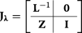
  in which $\mathbf {Z}=\frac {\partial \boldsymbol {\rho }}{\partial \text {vec}{(\boldsymbol {\Sigma }})}$. Assume:

  

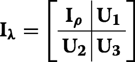
  By substituting I_λ and J_λ in I_θ, I_ρ=I is concluded. □

• Deriving SF:According to [44], when the induced FIM of the problem is I, the GWT detector coincides with the well-known Wald detector, and its statistic; can be written as

  $$ T_{\text{GWT}}=||\hat{\boldsymbol{\rho}}||^{2}=\widehat{\boldsymbol{\mu}^{H}\boldsymbol{\Sigma}^{-1}\boldsymbol{\mu}} \gtrless^{\mathcal{H}_{1}}_{\mathcal{H}_{0}} \eta $$

  (5)

  Interestingly, the GWT also coincides with the GLRT derived in [3].

Proposition 2

The GWT based classifier for (2) is UMEP in the C_α group for the special case of Σ=σ²I.

Proof

It can be proved that the GLR detector for (2) in the case of Σ=σ²I is UMPU detector [47]. As far as the GWT detector coincides with GLR detector (refer to (5)) according to Theorem 1, it is a UMEP classifier in the corresponding C_α □

Based on the preceding reasoning, using the GWT classifier for (3) is the optimal classifier in the C_α group at least for Σ=σ²I. On the other hand, when Σ has a different structure, the GWT can also be used as an asymptotically optimal classifier in the C_α group.

5 Error floor value evaluation

In this section, we want to evaluate the effect of the error floor on the classifier performance. In other words, we want to discuss which C_α group should be taken. It will be shown that under some circumstances, the C_α group is just a design parameter and α-selection is a trade-off between high SNR regime and low SNR regime performances.

Example 1

Assume a special case for (2) in which x obeys normal distribution, i.e., x∼N(ρ,1). Furthermore, the N-tuple observation vector x=[x₀,x₁,⋯,x_N−1]^T is also available. Consider the following binary classification problem:

$$ \left \{ \begin{array}{ll} \mathcal{C}_{0}: \rho =0\\ \mathcal{C}_{1}: \rho > 0 \end{array} \right. $$

(6)

in which ρ is unknown. For this simple problem, it can be easily seen that the corresponding hypothesis testing problem noted in Theorem 1 is itself. i.e.:

$$ \left \{ \begin{array}{ll} \mathcal{H}_{0}: \rho =0\\ \mathcal{H}_{1}: \rho > 0 \end{array} \right. $$

(7)

It is well-known that the UMP detector for (7) is $T_{\text {UMP}}(\mathbf {x})=\frac {1}{N}\sum _{n=0}^{N-1}x_{n}$[17]. Therefore, based on Theorem 1 using T_UMP as a classifier for (6) is the UMEP classifier in the C_α group. The error probability of the UMP-based classifier for (2) vs. ρ (which is a measure of SNR) for different error floor values (different C_α groups) is depicted in Fig. 1. As it is illustrated, increasing P_FA results in a higher error floor in large SNR regimes. But on the other hand, it results in a better error probability for lower values of SNR. We are going to evaluate this property in detail. Specifically, we would propose some sufficient conditions under which this property holds.

Fig. 1

Performance of the proposed classifier in Ex. 1 for different error floor values

Lemma 1

Suppose an arbitrary detector for (3) as T(.) for which we have : $\phantom {\dot {i}\!}\forall \boldsymbol {\rho } \in \Omega, \forall P_{\text {FA}}\in \mathbb {R}, \frac {\partial ^{2} P_{D}}{\partial P_{\text {FA}}^{2}} <0$. Furthermore, suppose $\forall P_{\text {FA}}, \exists \boldsymbol {\rho }^{*} \in \Omega : \frac {\partial P_{D}(\boldsymbol {\rho }^{*})}{\partial P_{\text {FA}}} >1$. Then for P_FA2<P_FA1, there exist ρ^∗∈Ω:P_e1(ρ^∗)<P_e2(ρ^∗).

Proof

Refer to Appendix B □

Remark 2

This lemma establishes some sufficient conditions guaranteeing that increasing the error floor value would lead to lower error probability for some SNR values. In the following, we are going to exploit the conditions stated in Lemma 1 to establish sufficient conditions in more general signal processing examples, i.e when the distribution of T(.) is an element of exponential family.

Definition 3

(Exponential Family [16]) Every pdf in the form of:

$$ f\left(x|\boldsymbol{\rho}\right)=h(x)\exp\left\{B(\boldsymbol{\rho})K(x)-A(\boldsymbol{\rho})\right\} $$

(8)

in which h(x), B(ρ), K(x), and A(ρ) are known functions is called the exponential family.

Theorem 2

Assume that in (3), the pdf of T(.) is distributed according to the exponential family. Then ∀P_FA2<P_FA1, there exists ρ^∗∈Ω for which we have $\phantom {\dot {i}\!}P_{e1({\boldsymbol {\rho ^{*}}})}<P_{e2({\boldsymbol {\rho ^{*}}})}$ if the two following conditions are held

• ∀ρ∈Ω:B(ρ)>B(ρ₀)

• $\forall \eta \in \mathbb {R}, \exists \boldsymbol {\rho }^{*}$ for which we have :

  $$ K(\eta) > \frac{A(\boldsymbol{\rho}^{*})-A(\boldsymbol{\rho_{0}})}{B(\boldsymbol{\rho}^{*})-B(\boldsymbol{\rho}_{0})} $$

  (9)

Proof

Refer to Appendix 7 □

Example 2

Suppose Ex. 1 again. It can be easily seen that T_UMP(x) is distributed as N(ρ,1). The normal distribution is an element of the exponential family with the following parameters:

$$\begin{array}{*{20}l} \begin{array}{ll} h(x)=\frac{1}{\sqrt{2\pi}}\exp\left\{-\frac{x^{2}}{2}\right\} \\ K(x)=x\\ A(\rho)=\frac{\rho^{2}}{2}\\ B(\rho)=\frac{\rho}{\sigma} \end{array} \end{array} $$

(10)

For this example, B(ρ)>B(ρ₀) leads to ρ>0. On the other hand applying (9) leads to:

$$ 2\eta > \rho $$

(11)

For every η>0 any ρ∈(0,η) satisfies (11). Therefore, for this examples as it was illustrated in Fig. 1 this property holds.

Corollary 1

Suppose g(ρ) is an SF for (3). Then in the asymptotic regime, i.e., when the number of samples for $\hat {g(\boldsymbol {\rho })}_{\text {ML}}$ approaches infinity, for any arbitrary P_FA2<P_FA1 there exist a ρ^∗ for which for any $\boldsymbol {\tilde {\rho }} \in (0,\boldsymbol {\rho }^{*})$ we have $P_{e1}(\boldsymbol {\tilde {\rho }}) <P_{e2}(\boldsymbol {\tilde {\rho }})$ assuming g(ρ₀)=0,

Proof

In asymptomatic regime the distribution of $\hat {g}(\boldsymbol {\rho })_{\text {ML}}$ can be modeled by N(g(ρ),V(ρ)) in which $V(\boldsymbol {\rho }) \triangleq \frac {\partial g(\boldsymbol {\rho })}{\partial \boldsymbol {\rho }}^{T} \mathbf {I}_{\boldsymbol {\rho }}^{-1}\frac {\partial g(\boldsymbol {\rho })}{\partial \boldsymbol {\rho }}$ and I_ρ is the FIM of f(m;ρ)[46]. Any normal distribution is an element of family distribution with the following parameter:

$$\begin{array}{*{20}l} \begin{array}{ll} K(\eta) =\frac{\eta}{\sqrt{V(\boldsymbol{\rho})}} \\ A(\boldsymbol{\rho}) =\frac{g^{2}(\boldsymbol{\rho}}{2V(\boldsymbol{\rho})} \\ B(\boldsymbol{\rho}) =\frac{g(\boldsymbol{\rho})}{\sqrt{V(\boldsymbol{\rho})}} \end{array} \end{array} $$

(12)

Applying conditions of Theorem 2

$$ 2\eta>g(\boldsymbol{\rho}) $$

(13)

Because g(.) is continuous, for every P_FA we can find a ρ which satisfies (13). □

Remark 3

Corollary 1 states that in asymptotic regimes, increasing error floor will result in a higher correct probability for lower SNR values for any SFET detector stratifying g(ρ₀)=0. According to (5), g(ρ)=0 and therefore asymptotically speaking, increasing the error floor for the GWT based classifier for (2), results in a lower error probability for some lower SNR values.

6 Results and discussion

Example 3

Consider the modulation classification problem in a multipath fading channel as $y_{i}=\sum _{l=0}^{L-1}h_{l}x_{i-l}+n_{i}$ in which h_i is the channel impulse response, x_is are the transmitted symbols, n_i represents the white Gaussian noise and L denotes the number of channel paths. Suppose that the classification is to be done from two different dictionaries D₁={BPSK, QPSK} and D₂={QPSK, 8PSK}. Based on [1] we can use $f_{1}\triangleq E\{y_{i}y_{i+q}\}$ and $f_{2} \triangleq E\{y_{i}^{2}y_{i+q}^{2}\}$ features for discriminating between D₁ and D₂ dictionaries. It is straightforward to see that for QPSK, $E\{x_{i}^{2}\}$ is zero but for BPSK it is not. Furthermore, $E\{x_{i}^{4}\}$ is zero for 8PSK and non-zero for QPSK. For estimating f₁ and f₂ we can use the sample mean estimator $\mathbf {z}_{f_{1}}(q) \triangleq \frac {1}{K}\sum _{k=0}^{K-1}y_{k}y_{k+q}, 0 \leq q < Q$ and $\mathbf {z}_{f_{2}}(q) \triangleq \frac {1}{K}\sum _{k=0}^{K-1}y_{k}^{2}y_{k+q}^{2}, 0 \leq q < Q$.

MC for the considered channel model based on f1 and f2 features can be modeled by the following binary classification problem (as the number of observations approaches infinity according to the central limit theorem)[1] $\mathcal {C}_{0}: \mathbf {z}_{f_{i}}\sim CN(\mathbf {0},\sigma ^{2}\mathbf {I})$ vs. $\mathcal {C}_{1}: \mathbf {z}_{f_{i}} \sim CN(\boldsymbol {\beta },\sigma ^{2}\mathbf {I})$ in which β is unknown which models the uncertainty due to fading channel and σ² is unknown representing the ambiguity of noise power and accuracy of the sample mean estimator. This problem is a special case of (2). Therefore, we can use the GWT classifier proposed for this problem. Assuming that N observation vectors are already available in the receiver and $\mathbf {y_{i}}=\left [y_{0}^{i},y_{1}^{i},\cdots,y_{Q-1}^{i}\right ]^{T}$ is the ith received observation vector, we have $\hat {\boldsymbol {\beta }}=\frac {1}{N}\sum _{i} \mathbf {y}_{i}$ and $\hat {\sigma }^{2}=\frac {1}{Q}tr\left \{\frac {1}{N}\sum _{i=0}^{N-1}(\mathbf {y}_{i}-\hat {\boldsymbol {\mu }})(\mathbf {y}_{i}-\hat {\boldsymbol {\mu }})^{H}\right \}$.

For the simulation results, P_FA is taken as 0.01, Q=9 and K=1000 otherwise noted. Furthermore, the Power Delay Profile (PDP) of the channel for different number of paths is taken as follows: L=4:P=[0.4615,0.3077,0.1538,0.0769],D=[0,20,30,32], L=3:P=[0.5,0.3333,0.1667],D=[0,20,30] and L=2:P=[0.6,0.4]D=[0,20] in which D and P vectors represent path gains and delays (in number of samples), respectively. The simulation results for D= {BPSK, QPSK} dictionary are illustrated in Figs. 2, 3, and 4. The simulation is conducted for different channel conditions and number of observation vectors. As it can be implied by the results, as the number of channel taps in a frequency selective fading channel increases, the error probability also increases. This is because the estimation error of parameters gets worse as the dimension of the observation vectors increases. On the other hand, increasing the number of observation vectors helps to increase the correct classification probability. In Fig. 3, the P_FA is depicted over different SNR values (noise power). As far as a CFAR detector is used for classification, it is expected that by changing the noise power, the P_FA remains constant. This phenomenon is verified through Monte Carlo simulation in Fig. 3. Furthermore, the effect of error floor on the classifier performance is depicted in Fig. 4 for C_0.01, C_0.05 and C_0.1 groups. As it is expected, taking a larger error floor leads to the lower SNR values performance improvement. On the other hand, the simulation results for D = {8PSK, QPSK} dictionary is depicted in Figs. 5 and 6. The classifier behaves as in the previous case. Increasing the number of channel taps results in the decrease of the correct probability of the classifier. Furthermore, as the number of observation vectors increases, the error probability decreases. The effect of error floor on the overall classifier performance is depicted in Fig. 6 for C_0.1, C_0.05, and C_0.01. In this case, also increasing the error floor results in a better performance in lower SNR regions.

Fig. 2

Error probability of the GWT classifier for different channel conditions and the number of observation vectors for D={BPSK,QPSK} dictionary

Fig. 3

False alarm probability of the GWT classifier for different number of channel taps, N=2 and D = {BPSK,QPSK}

Fig. 4

Effect of error floor value on the classifier performance for C_0.01, C_0.05 and C_0.1 for D₁={BPSK,QPSK}. Higher error floor values gain us in low-SNR value performance improvements

Fig. 5

Error probability of GWT classier for different channel conditions and number of observation vectors for D = {8PSK,QPSK} dictionary

Fig. 6

Effect of error floor value on the classifier performance for C_0.01, C_0.05 and C_0.1 for D₁ = {QPSK,8PSK}. Higher error floor values gain us in low-SNR value performance improvements

On the other hand, in order to better evaluate our proposed classifier against state of art solutions, the performance is compared against two Convolution Neural Network (CNN) classifiers. Adopting CNNs for modulation classification application is already proposed in the literature in [48–51]. The first selected CNN layout structure is given in Table 1. This structure is proposed by [50] which is somehow a similar structure used in [48]. The adopted classifier uses a CNN that consists of six convolution layers and one fully connected layer. Each convolution layer except the last is followed by a batch normalization layer, rectified linear unit (ReLU) activation layer, and a max-pooling layer. In the last convolution layer, the max-pooling layer is replaced with an average pooling layer. The output layer has softmax activation. A stochastic gradient descent with Momentum (SGDM) solver with a mini-batch size of 256 is used. The maximum number of epochs is set to 12 since a larger number of epochs provides no further training advantage. Furthermore, the initial learning rate is set to 0.02. On the other hand, the second CNN structure which is shown in Table 2 is adopted from [51] (very similar but not exactly identical). This CNN consists of two convolution layers and four fully connected layers. Each convolution layer and fully connected layer (except the lest one) is followed by a rectified linear unit (ReLU) activation layer and a max-pooling layer. The output layer has softmax activation. An SGDM solver is used and the maximum number of epochs is set to 8. Furthermore, the initial learning rate is set to 0.01.

Table 1 The first adopted CNN network layout

Table 2 The second adopted CNN network layout

The simulation results of the trained networks for L=4,D={BPSK,QPSK} are depicted in Fig. 7. The sample per symbol parameter is set to 1 and the number of samples fed to the CNN classifiers is taken in such a way that the observation elements available for the adopted classifiers (CNNs and our proposed one) are almost the same. For high SNR regimes (20 dB) the first CNN classifier performance reaches the probability of 98.2% for L=4 while the second CNN has an error floor in the high SNR regime around 0.15. The first CNN has a better performance in the high SNR regime while the second CNN network has better performance in the low SNR regime. Our proposed classifier has better performance compared to the first CNN performance for L=4,N=2. (e.g., 99% accuracy in SNR around 0 dB). However, in the low SNR regime, the second CNN has better performance while it has much more error floor against our proposed classifier. Furthermore, it should be noted that our proposed classifier has the optimal performance in C_0.05 group. Based on Theorem 1 proof, there may be a classifier outside C_0.05 which has better performance in some SNR points. However, it should be noted that selecting the CNN number of layers and its structure needs optimization which is definitely out of the scope of this paper. In other words, we may reach a better performance by changing the network structure. On other hand, the CNN classifiers are much more complex than our proposed classifier. Furthermore, our proposed classifier can control its error floor in order to boost its performance in low SNR regimes by changing the C_α group.

Fig. 7

Error probability of the GWT classfier and the CNN classifier for D={BPSK,QPSK} dictionary

Example 4

Consider Example 3 again. Now suppose that we want to classify in D = {BPSK, QPSK, 8PSK} dictionary. In this approach we convert the M-case classification problem into M binary classification problems. This procedure can be described by a decision tree as in Fig. 8. In each stage one of the candidates is tested; accordingly, the corresponding decision is taken until the final answer. At each node, a detector-based classifiers introduced in the previous sections for each binary decision-making is used. For classification, at first the discrimination is done between D₁ = {BPSK, QPSK} and then between D₂ = {QPSK,8PSK}. All of the detector’s parameters, i.e., K, Q, and P_FA are taken as in Example 3. The Monte Carlo simulation results are depicted in Fig. 9. In this case, also increasing the number of channel paths will result in a decrease in correct classification probability. On the other hand, increasing the number of observation vectors helps to increase the correct classification probability. Furthermore, it should be noted that for all cases, the error floor value is $\phantom {\dot {i}\!}P_{e}(\infty)=1-\frac {(1-P_{\text {FA}_{0}})(1-P_{\text {FA}_{1}})+(1-P_{\text {FA}_{0}})+P_{D_{0}}(\infty)}{3}$which equals 0.01 for the simulation parameter considered.

Fig. 8

Decision Tree of Ex. 4

Fig. 9

Error probability of the GWT classifier for different channel conditions and number of observation vectors for D={8PSK, QPSK, BPSK} dictionary

7 Conclusion

In this paper, the conditionally optimal solution for the classification problem when the observation vectors were from multivariate normal distribution was investigated. It was shown that the optimal classifier in the C_α group for such a problem is possible under some circumstances. Furthermore, when the optimal solution in the C_α group did not exist either, it was proved that taking a better detector for the corresponding hypothesis test problem leads to a better classifier. The GWT classifier was derived and was shown that it is optimal in the C_α group when the covariance matrix is a scaled identity matrix. The GWT classifier was applied to the AMC problem in the multipath channel. The simulation results verified the analytical findings. Furthermore, the superiority of our approach was evaluated against its alternative solution, i.e., CCN approach.

8 Appendix A: Proof of Theorem

Proof

First of all it can easily proved that P_MD(||ρ||→∞) approaches 0. Furthermore, as the tests are considered invariant they are all function of maximal invariant and the parameter space is function of induced maximal invariant [16] (Theorem 1). We prove that the induced maximal invariant with repect to the considred group of transformation, i.e., G is ρ because of the following two properties: 1- $\boldsymbol {\rho }\left (\bar {g}_{m}\left (\left (\boldsymbol {\mu },\boldsymbol {\Sigma }\right)\right)\right)=\boldsymbol {\rho }\left (\mathbf {L_{1}}\boldsymbol {\mu },\mathbf {L_{1}}\boldsymbol {\Sigma }\mathbf {L_{1}}^{H}\right)=\mathbf {L}^{-1}\mathbf {L_{1}}^{-1}\mathbf {L}_{1}\boldsymbol {\mu }=\mathbf {L}^{-1}\boldsymbol {\mu }= \boldsymbol {\rho }\left (\left (\boldsymbol {\mu },\boldsymbol {\Sigma }\right)\right), \forall \mathbf {L}_{1} \in \mathcal {L}$. 2- If ρ(θ₁)=ρ(θ₂) then $\boldsymbol {\mu }_{1} =\mathbf {L}_{1}\mathbf {L}_{2}^{-1}\boldsymbol {\mu }_{2}$, $\mathbf {L}_{1}\mathbf {L}_{2}^{-1}\boldsymbol {\Sigma }_{2}\mathbf {L}_{2}^{-H}\mathbf {L}_{1}^{H}=\boldsymbol {\Sigma }_{1}$ therefore $\bar {g}_{m}=\mathbf {L}_{1}\mathbf {L}_{2}^{-1}$ maps θ₂ to θ₁. To cmplete the proof we show that all classifiers in the C_α group are CFAR. We should show $\phantom {\dot {i}\!}P_{FA}(\boldsymbol {\mu _{1}}=0,\boldsymbol {\Sigma }=\boldsymbol {\Sigma }_{1}) =P_{\text {FA}}(\boldsymbol {\mu _{1}}=0,\boldsymbol {\Sigma }=\boldsymbol {\Sigma }_{2})$, ∀Σ₁,Σ₂. $P_{\text {FA}}(\boldsymbol {\mu _{1}}=0,\boldsymbol {\Sigma }_{1})= P_{\left (\boldsymbol {\mu _{1}}=0,\boldsymbol {\Sigma }_{1}\right)}\left \{T(\mathbf {x})\in A\right \}=P_{(\boldsymbol {\mu _{1}}=0,\boldsymbol {\Sigma }_{1})}\left \{T\left (g_{m}\left (\mathbf {x}\right)\right)\in A\right \}=P_{(\boldsymbol {\mu _{1}}=0,\boldsymbol {\Sigma }_{1})}\left \{g_{m}(\mathbf {x})\in T^{-1}(A)\right \}=P_{g_{m}\left (\boldsymbol {\mu _{1}}=0,\boldsymbol {\Sigma }_{1}\right)}\left \{\mathbf {x}\in T^{-1}(A)\right \}=P_{(\boldsymbol {\mu _{1}}=0,\boldsymbol {\Sigma _{2}})}\left \{T(\mathbf {x})\in A\right \}$. It should be noted that for every Σ,Σ₂, g_m exists and equals $\mathbf {L}_{1}\mathbf {L}_{2}^{-1}$. Therefore, every classifier in the C_α group is CFAR and as far as P_MD(||ρ||→∞) approaches 0, P_e(||ρ||→∞) forces P_FA to be α for all the classifiers in the C_α. Therefore, the UMP detector for (3) is the optimal classifier for (2) in the C_α group as it has the minimum missed detection probability with respect to a fixed false alarm probability. Furthermore, as all the classifiers in the C_α are unbiased, the UMPU detector for (3) is also the optimal solution because it can be easily proved that the unbiased detector for (3) is also an unbiased classifier for (2) (As far as the prior probability of different classes are equal). On the other hand, if T₁(.) has a better detection probability with respect to a predefined false alarm rate, it would have a better error probability in the corresponding C_α group because all the classifiers in the C_α has the same false alarm probability. □

9 Appendix B: Proof of Lemma 1

Proof

We should find ρ^∗:P_e1(ρ^∗)<P_e2(ρ^∗). Therefore we can write:

$$ \frac{1}{2}P_{\mathrm{FA1}}+\frac{1}{2}\left(1-P_{D1}(\boldsymbol{\rho}^{*}\right)<\frac{1}{2}P_{\mathrm{FA2}}+\frac{1}{2}\left(1-P_{D2}\left(\boldsymbol{\rho}^{*}\right)\right) $$

(14)

Then:

$$ \frac{P_{D1}(\boldsymbol{\rho}^{*})-P_{D2}(\boldsymbol{\rho}^{*})}{P_{\mathrm{FA1}}-P_{\mathrm{FA2}}}>1 $$

(15)

In the next steps, we prove that based on assumptions, (15) is satisfied. We can find ρ^∗ for P_FA2 in which we have $\frac {\partial P_{D}(\boldsymbol {\rho }^{*})}{\partial P_{FA}} >1$. Then based on mean value theorem [52], we can find P_FA3 in (P_FA2,P_FA1) interval for which we have:

$$ \frac{\partial P_{D}(\boldsymbol{\rho}^{*})}{\partial P_{\text{FA}(P_{\mathrm{FA3}})}}=\frac{P_{D1}(\boldsymbol{\rho}^{*})-P_{D2}(\boldsymbol{\rho}^{*})}{P_{\mathrm{FA1}}-P_{\mathrm{FA2}}} $$

(16)

On the other hand based on $\frac {\partial ^{2} P_{D}}{\partial P_{\text {FA}}^{2}} <0$, we can write $\frac {\partial P_{D}(\boldsymbol {\rho }^{*})}{\partial P_{\text {FA}(P_{\mathrm {FA3}})}}>1$. Therefore based on (16), (15) holds. □

10 Appendix C: Proof of Theorem 2

Proof

For detection probability we have:

$$ P_{D}(\boldsymbol{\rho})=\int_{\eta}^{\infty} f(\mathbf{m};\boldsymbol{\rho}) d\mathbf{m} $$

(17)

and for P_FA:

$$ P_{\text{FA}}=\int_{\eta}^{\infty} f(\mathbf{m};\boldsymbol{\rho}_{0})d \mathbf{m} $$

(18)

Using the chain formula we can write:

$$ \frac{\partial P_{D}}{\partial P_{\text{FA}}}=\frac{\partial P_{D}}{\partial \eta}\frac{\partial \eta}{\partial P_{\text{FA}}} $$

(19)

Using 19 and the Leibniz formula we can write:

$$ \frac{\partial P_{D}}{\partial P_{\text{FA}}}=\frac{f(\eta;\boldsymbol{\rho})}{f(\eta;\boldsymbol{\rho}_{0})} $$

(20)

in which η satisfies (18). Similarly, we can write:

$$ \frac{\partial^{2} P_{D}}{\partial P_{\text{FA}}^{2}}=-\frac{f'(\eta;\boldsymbol{\rho})f(\eta;\boldsymbol{\rho}_{0})-f'(\eta;\boldsymbol{\rho}_{0})f(\eta;\boldsymbol{\rho})}{f^{3}(\eta;\boldsymbol{\rho}_{0})} $$

(21)

Forcing $\frac {\partial ^{2} P_{D}}{\partial P_{\text {FA}}^{2}}<0$ and remembering that f(m;ρ)>0, we should have:

$$ \frac{f'(\eta,\boldsymbol{\rho})}{f'(\eta,\boldsymbol{\rho_{0}})}>\frac{f(\eta;\boldsymbol{\rho})}{f(\eta;\boldsymbol{\rho}_{0})} $$

(22)

Applying (22) on exponential family leads to:

$$ B(\boldsymbol{\rho}) > B(\boldsymbol{\rho}_{0}) $$

(23)

On the other hand we should have:

$$ \frac{f(\eta,\boldsymbol{\rho}^{*})}{f(\eta,\boldsymbol{\rho}_{0})}>1 $$

(24)

taking the assumption the exponential family distribution and some mathematical manipulation and based on monotone behavior of exponential function it leads to 9. □

References

M. Marey, O. A. Dobre, Blind modulation classification algorithm for single and multiple-antenna systems over frequency-selective channels. IEEE Signal Process. Lett.21(9), 1098–1102 (2014). https://doi.org/10.1109/LSP.2014.2323241.
M. Marey, O. A. Dobre, Blind modulation classification for alamouti stbc system with transmission impairments. IEEE Wirel. Commun. Lett.4(5), 521–524 (2015). https://doi.org/10.1109/LWC.2015.2451174.
A. V. Dandawate, G. B. Giannakis, Statistical tests for presence of cyclostationarity. IEEE Trans. Signal Process. 42(9), 2355–2369 (1994). https://doi.org/10.1109/78.317857.
E. Karami, O. A. Dobre, Identification of sm-ofdm and al-ofdm signals based on their second-order cyclostationarity. IEEE Trans. Veh. Technol.64(3), 942–953 (2015). https://doi.org/10.1109/TVT.2014.2326107.
Y. A. Eldemerdash, O. A. Dobre, B. J. Liao, Blind identification of sm and alamouti stbc-ofdm signals. IEEE Trans. Wirel. Commun.14(2), 972–982 (2015). https://doi.org/10.1109/TWC.2014.2363093.
E. Conte, A. De Maio, Distributed target detection in compound-gaussian noise with rao and wald tests. IEEE Trans. Aerosp. Electron. Syst.39(2), 568–582 (2003). https://doi.org/10.1109/TAES.2003.1207267.
A. De Maio, S. Iommelli, Coincidence of the rao test, wald test, and glrt in partially homogeneous environment. IEEE Signal Process. Lett.15:, 385–388 (2008). https://doi.org/10.1109/LSP.2008.920016.
I. S. Reed, X. Yu, Adaptive multiple-band cfar detection of an optical pattern with unknown spectral distribution. IEEE Trans. Acoust. Speech Signal Process.38(10), 1760–1770 (1990). https://doi.org/10.1109/29.60107.
M. E. Smith, P. K. Varshney, Intelligent cfar processor based on data variability. IEEE Trans. Aerosp. Electron. Syst.36(3), 837–847 (2000). https://doi.org/10.1109/7.869503.
A. Ghobadzadeh, A. Pourmottaghi, M. R. Taban, in 2011, 19th Iranian Conference on Electrical Engineering, IEEE. Clutter edge detection and estimation of field parameters in radar detection, (2011), pp. 1–6.
A. Ghobadzadeh, S. Gazor, M. R. Taban, A. Tadaion, S. M. Moshtaghioun, Invariance and optimality of cfar detectors in binary composite hypothesis tests. IEEE Trans. Signal Process.62(14), 3523–3535 (2014). https://doi.org/10.1109/TSP.2014.2328327.
F. C. Robey, D. R. Fuhrmann, E. J. Kelly, R. Nitzberg, A cfar adaptive matched filter detector. IEEE Trans. Aerosp. Electron. Syst.28(1), 208–216 (1992). https://doi.org/10.1109/7.135446.
K. J. Sangston, K. R. Gerlach, Coherent detection of radar targets in a non-gaussian background. IEEE Trans. Aerosp. Electron. Syst.30(2), 330–340 (1994). https://doi.org/10.1109/7.272258.
A. De Maio, L. Pallotta, J. Li, P. Stoica, Loading factor estimation under affine constraints on the covariance eigenvalues with application to radar target detection. IEEE Trans. Aerosp. Electron. Syst.55(3), 1269–1283 (2019). https://doi.org/10.1109/TAES.2018.2867699.
A. Aubry, A. De Maio, L. Pallotta, A. Farina, Radar detection of distributed targets in homogeneous interference whose inverse covariance structure is defined via unitary invariant functions. IEEE Trans. Signal Process.61(20), 4949–4961 (2013). https://doi.org/10.1109/TSP.2013.2273444.
E. L. Lehmann, J. P. Romano, Testing Statistical Hypotheses (Springer-Verlag, New York, 2005).
S. M. Kay, Fundamentals of Statistical Signal Processing: Detection Theory (Prentice-Hall PTR, Upper Saddle River, 1998). https://books.google.com/books?id=vA9LAQAAIAAJ.
O. A. Dobre, A. Abdi, Y. Bar-Ness, W. Su, Survey of automatic modulation classification techniques: classical approaches and new trends. IET Commun.1(2), 137–156 (2007). https://doi.org/10.1049/iet-com:20050176.
B. Tang, H. He, Q. Ding, S. Kay, A parametric classification rule based on the exponentially embedded family. IEEE Trans. Neural Netw. Learn. Syst.26(2), 367–377 (2015). https://doi.org/10.1109/TNNLS.2014.2383692.
A. K. Nandi, E. E. Azzouz, Algorithms for automatic modulation recognition of communication signals. IEEE Trans. Commun.46(4), 431–436 (1998). https://doi.org/10.1109/26.664294.
A. Swami, B. M. Sadler, Hierarchical digital modulation classification using cumulants. IEEE Trans. Commun.48(3), 416–429 (2000). https://doi.org/10.1109/26.837045.
B. G. Mobasseri, Digital modulation classification using constellation shape. Signal Process.80(2), 251–277 (2000). https://doi.org/10.1016/S0165-1684(99)00127-9.
Q. Zhang, O. A. Dobre, Y. A. Eldemerdash, S. Rajan, R. Inkol, Second-order cyclostationarity of bt-scld signals: Theoretical developments and applications to signal classification and blind parameter estimation. IEEE Trans. Wirel. Commun.12(4), 1501–1511 (2013). https://doi.org/10.1109/TWC.2013.021213.111888.
K. Hassan, I. Dayoub, W. Hamouda, M. Berbineau, Automatic modulation recognition using wavelet transform and neural networks in wireless systems. EURASIP J. Adv. Signal Process.2010(532898), 13 (2010).
M. L. D. Wong, A. K. Nandi, Automatic digital modulation recognition using artificial neural network and genetic algorithm. Signal Process.84(2), 351–365 (2004). https://doi.org/10.1016/j.sigpro.2003.10.019.Special Section on Independent Component Analysis and Beyond.
Y. Wang, T. Zhang, J. Bai, R. Bao, in 2011 Seventh International Conference on Intelligent Information Hiding and Multimedia Signal Processing. Modulation recognition algorithms for communication signals based on particle swarm optimization and support vector machines, (2011), pp. 266–269. https://doi.org/10.1109/IIHMSP.2011.31.
J. A. Sills, Maximum-likelihood modulation classification for psk/qam. IEEE Mil. Commun. Conf. Proc. (Cat. No.99CH36341). 1:, 217–2201 (1999). https://doi.org/10.1109/MILCOM.1999.822675.
K. Kim, A. Polydoros, in MILCOM 88, 21st Century Military Communications - What’s Possible?’. Conference Record. Military Communications Conference. Digital modulation classification: the bpsk versus qpsk case (IEEE, 1988), pp. 431–4362. https://doi.org/10.1109/MILCOM.1988.13427.
Wen Wei, J. M. Mendel, Maximum-likelihood classification for digital amplitude-phase modulations. IEEE Trans. Commun.48(2), 189–193 (2000). https://doi.org/10.1109/26.823550.
A. Polydoros, K. Kim, On the detection and classification of quadrature digital modulations in broad-band noise. IEEE Trans. Commun.38:, 1199–1211 (1990). https://doi.org/10.1109/26.58753.
P. Panagiotou, A. Anastasopoulos, A. Polydoros, in MILCOM 2000 Proceedings. 21st Century Military Communications. Architectures and Technologies for Information Superiority (Cat. No.00CH37155), 2. Likelihood ratio tests for modulation classification (IEEE, 2000), pp. 670–6742. https://doi.org/10.1109/MILCOM.2000.904013.
N. E. Lay, A. Polydoros, in Proceedings of 1994 28th Asilomar Conference on Signals, Systems and Computers, 2. Per-survivor processing for channel acquisition, data detection and modulation classification (IEEE, 1994), pp. 1169–11732. https://doi.org/10.1109/ACSSC.1994.471643.
N. E. Lay, A. Polydoros, in Proceedings of MILCOM ’95, 1. Modulation classification of signals in unknown isi environments (IEEE, 1995), pp. 170–1741. https://doi.org/10.1109/MILCOM.1995.483293.
K. M. Chugg, C. -S. Long, A. Polydoros, in Conference Record of The Twenty-Ninth Asilomar Conference on Signals, Systems and Computers, 2. Combined likelihood power estimation and multiple hypothesis modulation classification (IEEE, 1995), pp. 1137–11412. https://doi.org/10.1109/ACSSC.1995.540877.
L. Hong, K. C. Ho, in MILCOM 2000 Proceedings. 21st Century Military Communications. Architectures and Technologies for Information Superiority (Cat. No.00CH37155), 2. Bpsk and qpsk modulation classification with unknown signal level (IEEE, 2000), pp. 976–9802. https://doi.org/10.1109/MILCOM.2000.904076.
L. Hong, K. C. Ho, in MILCOM 2002. Proceedings, 1. Antenna array likelihood modulation classifier for bpsk and qpsk signals (IEEE, 2002), pp. 647–6511. https://doi.org/10.1109/MILCOM.2002.1180521.
F. Hameed, O. A. Dobre, D. C. Popescu, On the likelihood-based approach to modulation classification. IEEE Trans. Wirel. Commun.8(12), 5884–5892 (2009). https://doi.org/10.1109/TWC.2009.12.080883.
A. Ghobadzadeh, Optimal and suboptimal signal detection-on the relationship between estimation and detection theory. PhD thesis, Queen’s University at Kingston (2015).
E. Conte, A. De Maio, C. Galdi, Cfar detection of multidimensional signals: an invariant approach. IEEE Trans. Signal Process.51(1), 142–151 (2003). https://doi.org/10.1109/TSP.2002.806554.
J. R. Gabriel, S. M. Kay, On the relationship between the glrt and umpi tests for the detection of signals with unknown parameters. IEEE Trans. Signal Process.53(11), 4194–4203 (2005). https://doi.org/10.1109/TSP.2005.857043.
A. DeMaio, Generalized cfar property and ump invariance for adaptive signal detection. IEEE Trans. Signal Process.61(8), 2104–2115 (2013). https://doi.org/10.1109/TSP.2013.2245662.
A. A. Tadaion, M. Derakhtian, S. Gazor, M. M. Nayebi, M. R. Aref, Signal activity detection of phase-shift keying signals. IEEE Trans. Commun.54(8), 1439–1445 (2006). https://doi.org/10.1109/TCOMM.2006.878830.
S. M. Kay, J. R. Gabriel, Optimal invariant detection of a sinusoid with unknown parameters. IEEE Trans. Signal Process.50(1), 27–40 (2002). https://doi.org/10.1109/78.972479.
M. Naderpour, A. Ghobadzadeh, A. Tadaion, S. Gazor, Generalized wald test for binary composite hypothesis test. IEEE Signal Process. Lett.22(12), 2239–2243 (2015). https://doi.org/10.1109/LSP.2015.2472991.
A. Ghobadzadeh, S. Gazor, M. R. Taban, A. A. Tadaion, M. Gazor, Separating function estimation tests: A new perspective on binary composite hypothesis testing. IEEE Trans. Signal Process.60(11), 5626–5639 (2012). https://doi.org/10.1109/TSP.2012.2211594.
S. M. Kay, Fundamentals of Statistical Signal Processing. Estimation Theory.
D. Birkes, Generalized likelihood ratio tests and uniformly most powerful tests. Am Stat.44(2), 163–166 (1990).
T. J. O’Shea, T. Roy, T. C. Clancy, Over-the-air deep learning based radio signal classification. IEEE J. Sel. Top. Signal Process.12(1), 168–179 (2018).
X. Liu, D. Yang, A. E. Gamal, in 2017 51st Asilomar Conference on Signals, Systems, and Computers. Deep neural network architectures for modulation classification (IEEE, 2017), pp. 915–919.
Modulation Classification with Deep Learning. https://www.mathworks.com/help/deeplearning/ug/modulation-classification-with-deep-learning.html.
T. O’Shea, J. Hoydis, An introduction to deep learning for the physical layer. IEEE Trans. Cogn. Commun. Netw.3(4), 563–575 (2017). https://doi.org/10.1109/TCCN.2017.2758370.
H. Flanders, J. J. Price, Calculus with Analytic Geometry (Elsevier Inc, Amsterdam, 1985).
Acknowledgements
We acknowledge the support of Ali Akbar Tadaion Taft from Yazd University for his critical remarks.
Funding
The work is not funded by any private grant.
Author information
Authors and Affiliations
Contributions
MN conceived the study and conducted the experiments. HKB supervised the study. MN wrote the paper and HKB reviewed and edited the manuscript. The authors read and approved the final manuscript.
Corresponding author
Ethics declarations
Consent for publication
Informed consent was obtained from all authors included in the study.
Competing interests
The authors declare that they have no competing interests.
Additional information
Publisher’s Note
Springer Nature remains neutral with regard to jurisdictional claims in published maps and institutional affiliations.
Rights and permissions
Open Access This article is licensed under a Creative Commons Attribution 4.0 International License, which permits use, sharing, adaptation, distribution and reproduction in any medium or format, as long as you give appropriate credit to the original author(s) and the source, provide a link to the Creative Commons licence, and indicate if changes were made. The images or other third party material in this article are included in the article’s Creative Commons licence, unless indicated otherwise in a credit line to the material. If material is not included in the article’s Creative Commons licence and your intended use is not permitted by statutory regulation or exceeds the permitted use, you will need to obtain permission directly from the copyright holder. To view a copy of this licence, visit http://creativecommons.org/licenses/by/4.0/.
About this article
Cite this article
Naderpour, M., Bizaki, H.K. Conditionally optimal classification based on CFAR and invariance property for blind receivers. EURASIP J. Adv. Signal Process. 2021, 14 (2021). https://doi.org/10.1186/s13634-021-00723-9
Received:
Accepted:
Published:
DOI: https://doi.org/10.1186/s13634-021-00723-9