Target-driven obstacle avoidance algorithm based on DDPG for connected autonomous vehicles

Abstract

In the field of autonomous driving, obstacle avoidance is of great significance for safe driving. At present, in addition to traditional obstacle avoidance algorithms including VFH algorithm, artificial potential field method, a large number of related researches are focused on algorithms based on vision and neural networks. Researches on these algorithms have achieved some results, and some of which have completed real road tests. However, most of algorithms consider only local environmental information which may cause local optimum in complex driving environments. Therefore, it is necessary to consider the environmental information beyond the sensor's perceptual ability for autonomous driving in complex environment. In the network-assisted automated driving system, networked vehicles can obtain road obstacles’ and condition information through roadside sensors and mobile network, so as to gain extra sensing ability. Therefore, network-assisted automated driving is of great significance in obstacle avoidance. Under this background, this paper presents an automatic driving obstacle avoidance strategy combining path planning and reinforcement learning. At first, a global optimal path is planned through global information, then merge the global optimal path and vehicle information into a vector. Use this vector as input of reinforcement learning neural network and output vehicle control signals to follow optimal path while avoiding obstacles.

1 Introduction

With the continuous development of science and technology, artificial intelligence has gradually entered all aspects of human life, as well as in the field of transportation. In the last decade, the development of automatic driving has advanced by leaps and bounds. With the participation of many large companies and the continuous improvement of automatic driving related standards, automatic driving technology is developing in a better and better direction. For instance, the projects on automatic driving done by Google and Tesla are single vehicle automatic driving [1]. This automatic driving mode only relies on the sensor equipment carried by the vehicle to sense the surrounding environment and drive according to the planned route. "Networking" and "intelligence" have become a new generation of development direction of China's automobile industry. Specifically, the network connected automatic driving vehicle is equipped with advanced on-board sensors, controllers and other devices. It is connected to the network through the mobile network access point to obtain the automatic driving auxiliary information, the other intelligent information, the vehicle status information and the road condition information sent by the network in real time. The network connected automatic driving technology integrates modern communication and network technologies, realizes the interaction of people, vehicles, roads, networks and other information, and provides safe, comfortable, energy-saving and efficient driving capabilities. It is a new generation of autonomous driving technology with great potential, and it is also the future development trend of autonomous driving [2].

In automatic driving, the first thing to be considered is safety. Obstacle avoidance should be the most basic function of automatic driving. At present, the sensing equipment of the automatic driving car mainly includes camera, laser radar, millimeter wave radar and ultrasonic radar. In terms of obstacle avoidance, the obstacle avoidance strategies are also different according to the vehicle intelligence level. When the vehicle level is L2 or L3, the vehicle has the function of collision warning and emergency braking when the distance is too close. After the vehicle reaches L4 level, it has the functions of emergency braking and bypassing obstacles. Obstacle avoidance is a complex comprehensive decision-making task. At present, the obstacle avoidance methods using traditional methods and reinforcement learning methods have been studied and practiced.

Although there has been a lot of research on obstacle avoidance algorithms for automatic driving, there are still some problems and challenges:

• The problems falling into local optimization in the process of avoiding obstacles

In the case of single vehicle automatic driving, because the vehicle can only obtain the obstacle information around the vehicle through the on-board sensor, the vehicle control has the characteristics of local optimization. The goal-driven obstacle avoidance task includes two parts: moving to the target point and obstacle avoidance. In the vehicle control, these two parts could be considered comprehensively. However, the system with local optimal control characteristics would pay too much attention to the immediate interests and could not understand the long-term interests. Specifically, if there are obstacles near the vehicle, the vehicle will think more about the obstacles around it. Only when there are no obstacles around, more consideration will be given to move to the target point [3]. In order to avoid vehicles falling into local optimization, it is very significant to obtain comprehensive information and carry out path planning.

• Vehicle model needs to be considered in vehicle control

In the simulation environment or the real environment, the vehicle model needs to be considered. According to the finite integral form of whether the position coordinates could be obtained, the vehicle model could be divided into complete constraint model and non-complete constraint model [4]. Compared with nonholonomic constraint model, the solution of holonomic constraint model is relatively simple. In the automatic control theory, when there are the paths to be followed and the surrounding obstacle information, this task [5] could be handled by a variety of vehicle control algorithms, but this involves a lot of automatic control theory knowledge, which is difficult to deploy the algorithms. In order to solve the problem that the automatic control algorithm is too complex, reinforcement learning could be adopted for vehicle control.

• When the vehicle follows the global path, it will be affected by dynamic obstacles

The global path is obtained by considering static obstacles. If there are dynamic obstacles in the environment, the vehicle must try to avoid static and dynamic obstacles when following the global path. If the traditional algorithm is used, the size, distribution and moving speed of obstacles and the relative position of targets will have a great impact on vehicle control [6,7,8], and the control mode is more complex. If the reinforcement learning method is used, the reinforcement learning model needs to be considered for the two tasks of "path following" and "obstacle avoidance." Compared with single-task reinforcement learning, this multi-task reinforcement learning training is more difficult and the weight of each task needs to be comprehensively considered [9].

2 Related work

In this section, several related issues, including studies on path planning algorithm, obstacle avoidance algorithm, are reviewed, respectively.

• (A) Issues on Path Planning Algorithm

The path planning algorithm is divided into graph-based path planning algorithm [10] and sampling-based path planning algorithm [11]. Graph-based path planning algorithm is a complete algorithm. Namely, if there is a feasible path from the starting point to the target point, the solution must be obtained. If there is no solution, there must be no path from the starting point to the target point. This kind of algorithm is usually planned on a grid network map. At present, the commonly used algorithms are depth-first prime search algorithm, breadth-first search algorithm, Dijkstra algorithm and A* algorithm. Being different from map-based path planning algorithm, this type of algorithm does not require rasterization of the map, but randomly sets some sampling points in the map and uses these sampling points to abstract the actual map to perform path planning. Compared with the graph-based path planning algorithm, the sampling-based path planning algorithm has a faster calculation speed, but the cost of the generated path may be higher, and it would cause a situation of "no solution." Such algorithm is generally widely used in high-dimensional planning problems. At present, the commonly used sampling-based path planning algorithms include PRM algorithm, RRT algorithm and their improved algorithm.

The literature [12] shows comparing the time complexity, the graph-based path planning algorithm is more efficient than the sampling-based path planning algorithm, when the number of nodes is the same. However, when the granularity of rasterization is considered, the node number of the graph-based path planning algorithm is much larger than that of the sampling-based path planning algorithm. Therefore, the actual situation is that the sampling-based path planning algorithm has higher calculation efficiency. The literature [13] shows when the graph-based path planning algorithm is considered and the map in the form of a two-dimensional matrix is rasterized, the vehicle model constraints are not considered during path planning. Therefore, the obstacle avoidance effect is affected by the rasterization granularity and the adopted vehicle model. It is difficult to clearly analyze the obstacle avoidance effect.

• (B) Obstacle Avoidance Algorithm

The Vector Field Histogram algorithm [14, 15] is a real-time motion planning algorithm that uses sensors on the intelligent agent to detect the surrounding environment, generate obstacle distance histograms, and use the histogram to perform target-driven obstacle avoidance. In practice, the VFH algorithm has been proven to be fast and reliable, especially when traversing densely populated obstacle routes. However, the VFH algorithm only considers local obstacle information and belongs to a local path planning algorithm. The artificial potential field method [16] is an algorithm for avoiding obstacles in analogy to the phenomenon of "homogeneous phase exclusion and specific phase absorption" in an analogous electric field. At present, there are many obstacle avoidance algorithms based on reinforcement learning, which can be roughly divided into the following four categories: obstacle avoidance in a static environment, obstacle avoidance in a dynamic environment, target-driven obstacle avoidance in a static environment [17, 18] and target-driven obstacle avoidance in the dynamic environment [9]. The first two do not have the task of "reaching the goal." When setting the reward function, the closer is to the obstacle, the greater the penalty is. The farther is from the obstacle, the smaller the penalty is. The latter two include the task of "reaching the goal." When setting the reward function, it is necessary to weight the distance from the target and the distance from the obstacle. In most papers, goal-driven obstacle avoidance in a dynamic environment involves the problem of multi-agent obstacle avoidance.

• (C) Wireless communication technology in autonomous driving

In the auto-drive network, the literature [19] shows A novel market-based solution is proposed for interference management in MSS by introducing an elastic price mechanism that it can be used in the networking access of automatic driving. The literature [20] shows the clustering algorithm and cluster head alternation are proposed to improve transmission performance and ensure energy balance, respectively. The literature [21] shows the power allocation and network selection for the integrated IIoT are proposed to decrease the transmission cost. The above technology can provide reliable communication guarantee for automatic driving.

After comparing the completeness, computational efficiency, and obstacle avoidance effects of several path planning algorithms, the RRT* algorithm is finally selected as the path planning algorithm for this project, and then, the specific content of the RRT* algorithm is described. Secondly, two traditional obstacle avoidance algorithms and an obstacle avoidance algorithm based on reinforcement learning are introduced. By comparing the advantages and limitations of the two types of algorithms, the obstacle avoidance algorithm based on reinforcement learning is selected as the obstacle avoidance algorithm for this project.

3 Target-driven obstacle avoidance algorithm based on DDPG

3.1 The establishment of scenarios and models

3.1.1 Vehicle model

In this project, a fully constrained vehicle kinematics model is adopted. The description of the vehicle in the scene includes coordinates, speed magnitude and speed direction. The symbols are shown in Fig. 1.

Fig. 1

Vehicle status information

It is assumed that the simulation time interval of each step is $\Delta T$. The vehicle moves in a straight line at a constant speed in each time. The control variables of the vehicle are the longitudinal acceleration and the angular acceleration in the velocity direction. Therefore, within the simulation time interval of one step, the following equation is satisfied:

$$\begin{gathered} V_{t + 1} = V_{t} + \alpha \Delta T \hfill \\ \theta_{t + 1} = \theta_{t} + \beta \Delta T \hfill \\ xCar_{t + 1} = xCar_{t} + V_{t + 1} \Delta T\cos (\theta_{t + 1} ) \hfill \\ yCar_{t + 1} = yCar_{t} + V_{t + 1} \Delta T\sin (\theta_{t + 1} ) \hfill \\ \end{gathered}$$

(1)

The contour of the equivalent vehicle is approximated according to the encircling circle method. The 11 laser rangefinders are installed at equal angular intervals in front of the vehicle to measure the distances of obstacles in 11 different directions. The vehicle equivalent model is shown in Fig. 2.

Fig. 2

Vehicle equivalent model

3.1.2 Training scenario

The tasks to be completed by reinforcement learning are: reaching the target point and avoiding obstacles. The training scene can include dynamic obstacles and static obstacles. However, because the reinforcement learning algorithm has Markov characteristics, it is impossible to judge the movement direction and speed of the currently detected obstacles from the state information of the vehicle. If dynamic obstacles are contained, the obstacle avoidance behavior of the vehicle will be affected by the movement state of the currently detected obstacle, resulting in different evaluations when the vehicle performs the same action in the same state. Namely, the Q function is unstable.

Therefore, in this project, the training scene could be the scene with only static obstacles and use the encircling circle method to approximate the contour of the obstacle, as shown in Fig. 3.

Fig. 3

Training scene

3.2 Neural network design based on DDPG

3.2.1 Overview of DDPG algorithm

DDPG (Deep Deterministic Policy Gradient) algorithm [18] is a model free, off-policy reinforcement learning algorithm that can be used to solve continuous state space and continuous action space problems. DDPG is based on actor-critic, which includes both value function network (critic) and policy network (actor).

The DDPG algorithm has many advantages to adopt a deterministic strategy network and update the strategy network using strategy gradients. This enables the network to handle high-dimensional continuous actions. The introduction of experience playback arrays increases the utilization of data to; adopt dual network updates of the target network and the current network. This makes the algorithm easier to converge. The target network adopts the soft update method, which increases the stability of the algorithm.

3.2.2 DDPG algorithm principle

DDPG uses a neural network to approximate the value function. This value function network is also called a critic network. Its input is action and state value $[a,s]$, and its output is $Q(s,a)$. There is also a neural network to approximate the strategy function. This strategy network is also called an actor network. Namely, its input is a state $s$, and its output is an action $a$.

The critic network uses the gradient descent method to minimize the loss function and update the network parameters. The specific method is as follows. $N$ in the formula is the size of the mini-batch:

$$\begin{aligned} & y_{i} = r_{i} + \gamma Q(s_{i + 1} ,\mu (s_{i + 1} |\theta^{\mu } )|\theta^{Q} ) \\ & Loss = \frac{1}{N}\sum\limits_{i} {(y_{i} - Q(s_{i} ,a_{i} |\theta^{Q} ))^{2} } \\ \end{aligned}$$

(2)

The actor network follows the chain rule and updates the network parameters by analogy with the strategy gradient algorithm. The specific methods are as follows:

$$\begin{aligned} & \nabla_{{\theta^{\mu } }} J \approx {\mathbf{E}}_{{s_{t} \sim \rho^{\beta } }} \left[ {\nabla_{{\theta^{\mu } }} Q(s,a|\theta^{Q} )|_{{s = s_{t} ,a = \mu (s_{t} |\theta^{\mu } )}} } \right] \\ & \quad \quad \quad = {\mathbf{E}}_{{s_{t} \sim \rho^{\beta } }} \left[ {\nabla_{a} Q(s,a|\theta^{Q} )|_{{s = s_{t} ,a = \mu (s_{t} )}} \nabla_{{\theta^{\mu } }} \mu (s|\theta^{\mu } )|_{{s = s_{t} }} } \right] \\ \end{aligned}$$

(3)

DDPG requires samples to be independently and identically distributed, so it is necessary to use experience playback arrays for mini-batch learning. In addition, for reference to DQN's dual network technology, DDPG divides both the critic network and the actor network into the target network and the current network. And the soft update method is used to greatly increase the stability of the network.

3.2.3 DDPG algorithm steps

See Algorithm 4.

3.2.4 Design of neural network

• (A) Neural network structure

Figure 4 shows the actor network built in this article, including 3 hidden layers, which are all fully connected networks. We set the fully connected layer Fc1 to 300 neurons, set the fully connected layer Fc2 to 400 neurons, and set Fc3 to 300 neurons. The number of nodes in the output layer is the same as the action dimension. The activation function of the hidden layer selects the relu function, and the activation function of the output layer is tanh. The network input is the state $s$, and the output is the action $a$.

Fig. 4

Actor network structure

Figure 5 shows the critic network built in this article, including 2 hidden layers, which are all fully connected networks. The activation functions are all relu. The fully connected layer Fc1 is connected to the input state $s$ and contains 300 neurons. The fully connected layer Fc2 is connected to the input action $a$ and contains 300 neurons. The Fc1 output and the Fc2 output are added to the fully connected layer Fc3 and Fc3 contains 100 Neuron. The output layer contains 1 neuron to represent $Q(s,a)$ for linear activation.

Fig. 5

Critic network

• (B) Network parameter setting

The size of the experience replay array is $10^{5}$. Generally speaking, the larger the experience replay array is, the longer the training data could be used. The data utilization rate would be improved. However, if the reinforcement learning network generates more garbage data during the training process, an excessively large experience playback array will cause the garbage data to be learned multiple times, thereby affecting the final effect. In this project, because the obstacles in the training environment are randomly generated, it is possible that the target point cannot be reached. Such data are garbage data. In order to reduce the impact of garbage data, we set the experience playback array size to be smaller.

The discount factor is set to 0.98. The empirical formula ${1 \mathord{\left/ {\vphantom {1 {1 - \gamma }}} \right. \kern-\nulldelimiterspace} {1 - \gamma }}$ represents the number of steps considered in the future. There are some special situations in this project. There are obstacles near the target point, or the target point is reached through obstacles. At this time, approaching obstacles is able to reach the target point in the future. Therefore, during training, we need to consider the impact of the next few steps as much as possible. However, if $\gamma$ is too large, it may make the algorithm difficult to converge. Therefore, $\gamma$ is set to 0.98 to consider the impact of the next 50 steps.

The batch size is set to 32. The reason is similar to the setting of the experience playback array. If more garbage data will be generated during training, too large batch size will increase the impact of garbage data on the result. So, the bath size should be small he. However, too small batch size may cause the algorithm to converge to the local optimum, so the batch size is set to 32 here.

We take Gaussian random process as the exploration noise. The actions must be normalized. The standard deviation of the initial Gaussian noise is 1. After each iteration, the standard deviation of the Gaussian noise becomes 0.99 times of the original. Generally speaking, continuous and inertial motions are all explored by adding Gaussian noise. Here, we take the general method.

The soft update coefficients $\tau$ of the actor network and the critic network are both 0.01. In the DDPG algorithm, in order to ensure the stability of the algorithm, the value $\tau$ is generally small and its value is 0.1 or 0.01. In some cases, the value $\tau$ of critic will be slightly larger than the value $\tau$ of actor. Here, the values $\tau$ of the two networks are set to be the same.

Both the actor network and the critic network are updated with the Adam optimizer. The learning rate of the actor network is 0.0001, and the learning rate of the critic network is 0.0002. The learning rate of the Adam optimizer is generally recommended to be 0.0001. In this project, the actor network is set according to the recommended value. The critic network needs to converge as soon as possible, so the learning rate can be set slightly larger.

4 Methods and experimental

4.1 Simulation environment

There are only stationary obstacles in the environment of this experiment. It is assumed that the equivalent circle radius of all obstacle contours is the same as the equivalent circle radius of the vehicle $rCar = rObstacle = 0.5\;{\text{m}}$. The test scene is a two-dimensional plane of 25 m*25 m, with the abscissa $x \in [0,25]\;{\text{m}}$ and the vertical coordinate $y \in [0,25]\;{\text{m}}[0,25]$$\;{\text{m}}$. The target area is a circle, and the radius is $endR = 0.1\;{\text{m}}$. In the initial state, the vehicle position and direction are randomly generated, and the speed is 0. The target area is randomly generated. The obstacles are randomly generated without overlap. The simulation time interval is $\Delta T = 0.01\;{\text{s}}$. The number of training rounds is 300, and each round has a maximum of 1000 time steps. If $done = true$, then the round is stopped.

• 1. Status. The description of the state in this project includes the data received by the vehicle-mounted sensor, the positional relationship of the vehicle relative to the target area, and the speed and direction information of the vehicle. It is composed of these three parts. There are 11 vehicle-mounted laser rangefinders, which are evenly distributed within 180° in front of the car. The maximum detection distance of each rangefinder is $maxSensorDis = 4\;{\text{m}}$. The 11 laser rangefinders form the sensor vector $sensors = (sensor_{1} ,sensor_{2} , \ldots ,sensor_{11} )$ in the order from the front left side of the car to the front right side of the car. The position relationship of the vehicle relative to the target is expressed in the form of polar coordinates, with the center of the vehicle as the pole and the $x$ axis of the two-dimensional plane as the direction of the polar axis, as shown in Fig. 6. Thereinto, the polar diameter of the vehicle is $dg$ and the polar angle is $cgAngle \in ( - \pi ,\pi ]$. The speed of the vehicle is $vCar \in [0,10]$, and the speed direction is $vthetaCar \in ( - \pi ,\pi ]$. The above three parts are spliced into a 15-dimensional vector, and there into the values are normalized to obtain the state vector:

  $$s = \left( {\frac{dg}{{maxSensorDis}},\frac{cgAngle}{\pi },\frac{vCar}{{vMax}},\frac{vthetaCar}{\pi },\frac{sensors}{{maxSensorDis}}} \right)$$

  (4)

  Fig. 6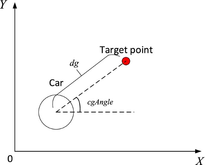

  

  The position of the vehicle relative to the target

• 2. Action $a$. According to the previous introduction to the vehicle model, the control quantity is a two-dimensional row vector composed of longitudinal acceleration $\alpha \in [ - \frac{{vMax^{2} }}{2*rCar},\frac{{vMax^{2} }}{2*rCar}]$ and angular acceleration $\beta \in [ - \frac{\pi }{18},\frac{\pi }{18}]$ in the direction of velocity. We use the two-dimensional normalized action vector outputted by the neural network to generate the vehicle control quantity, namely:

  $$(\alpha ,\beta ) = a\left( {\begin{array}{*{20}l} {\frac{{vMax^{2} }}{2*rCar}} \hfill & 0 \hfill \\ 0 \hfill & {\frac{\pi }{18}} \hfill \\ \end{array} } \right)$$

  (5)

• 3. Training is terminated $done$. There are three types of training termination situations, which are reaching the target area, colliding with an obstacle, and exceeding the boundary of the area. When training is terminated, set $done = true$, otherwise $done = false$.

• 4. Reward $r$. The overall reward function consists of three parts, which is distance reward from the target point, distance reward from obstacles, and training termination reward. The overall formula is shown in Eq. 5. $reward_{1} (s,a)$, $reward_{{2}} (s,a)$ and $reward_{{3}} (s,a)$ are shown in formulas 6, 7, and 8, respectively. Among them, $dgOld$ is the value $dg$ before the action $a$.

  $$r = reward_{1} (s,a) + reward_{2} (s,a) + reward_{3} (s,a) - 1$$

  (6)
  $$reward_{1} = \left\{ {\begin{array}{*{20}l} { - 3,} \hfill & {dg \ge dgOld} \hfill \\ {0,} \hfill & {dg < dgOld} \hfill \\ \end{array} } \right.$$

  (7)
  $$reward_{2} (s,a) = - \sum\limits_{i = 1}^{11} {\min \left( {\frac{10}{{sensor_{i} }} - \frac{10}{{maxSensorDis}},15} \right)}$$

  (8)
  $$reward_{3} (s,a) = \left\{ {\begin{array}{*{20}l} {500,} \hfill & {{\text{Reach}}\,{\text{the}}\;{\text{target}}\;{\text{area}}} \hfill \\ { - 100,} \hfill & {{\text{Collision}}\;{\text{with}}\;{\text{obstacles}}} \hfill \\ { - 100,} \hfill & {{\text{Cross}}\,{\text{the}}\;{\text{border}}} \hfill \\ \end{array} } \right.$$

  (9)

4.2 Performance analysis

The obstacle avoidance performance is tested under 10 obstacles, 20 obstacles and 30 obstacles. The test process starts from initializing vehicle, obstacles, and target location until the vehicle reaches the target area. The position of the car is displayed at each moment on the map, and the final vehicle obstacle avoidance effect is shown in Fig. 7.

Fig. 7

10,20.30 obstacles are contained

The target points in the picture are red dots, the connected circles are the vehicle's trajectory, and the separated circles are stationary obstacles. The 11 lines in front of the car are the distances detected by the laser rangefinder. When there is an obstacle blocking the laser rangefinder, the detected distance becomes shorter.

From the test results in the above three scenarios, it can be seen that the number of obstacles increases, and the obstacle avoidance behavior of the vehicle is more complicated. However, in the end, it can reach the target area smoothly. The obstacle avoidance effect based on reinforcement learning in a static environment is quite excellent, and it can complete the two tasks of obstacle avoidance and reach the target at the same time. However, the above obstacle avoidance method only takes for the local obstacle information and yet does not take for the global obstacle information. In some special scenarios, it will fall into the local optimal value and cannot reach the end point, as shown in Fig. 8.

Fig. 8

Falling into a local optimum

In order to solve the problem of falling into local optimum in the obstacle avoidance algorithm of traditional reinforcement learning, this paper will propose a dynamic path-following automatic driving scheme combined with path planning in the fourth chapter. By the global obstacles and the target area information being considered, the vehicle is prevented from falling into the local optimum, and the vehicle is guided to drive along the global optimum path.

5 Design and implementation of automatic driving obstacle avoidance scheme based on dynamic path following

5.1 Path planning realization

For the path planning algorithm in this paper, the RRT* algorithm is selected and has been introduced in detail in Chapter 2. The extend function of the RRT* algorithm includes the design of the cost function and the collision detection function. The specific selection scheme of these two functions will be introduced below.

5.1.1 The choice of cost function

The meaning of the cost function is to represent the cost from one point to another point. It is represented by symbol $c$ in the extend algorithm. The choice of the cost function can directly affect the performance of the RRT* algorithm path planning. However, setting a cost function is very appropriate to the actual problem. The difficulty is no less than that of designing a path planning algorithm. In addition, the cost function will also have a great impact on the convergence rate of the algorithm. Common cost functions include the Euclidean distance between two points, the weighted sum of different terrain lengths, and the cost function for energy consumption.

The simulation environment of this project is a fully constrained car model under the same terrain. There is no need to consider energy consumption. Therefore, choosing Euclidean distance as the cost function can accelerate the convergence of the algorithm and is easy to understand, as shown in Eq. 10. The total cost from the starting point to a certain point is derived as Eq. 11.

$$c(Line(x_{1} ,x_{2} )) = \left\| {x_{1} - x_{2} } \right\|$$

(10)

$${\text{Cos}} t(x) = \left\{ {\begin{array}{*{20}l} {{\text{Cos}} t(xParent) + c(Line(xParent,x)),} \hfill & {x \ne root} \hfill \\ {0,} \hfill & {x = root} \hfill \\ \end{array} } \right.$$

(11)

5.1.2 Vehicle and obstacle collision detection

In the RRT* algorithm, collision detection between cars and obstacles is required. A reasonable collision detection algorithm is very important to ensure the safety of car driving. Common collision detection methods include AABB enclosing box method and enclosing circle method [9]. This project uses the relatively simple calculation of the enclosing circle method. The specific implementation steps are as follows:

If the irregular object is converted to a circle with a slightly larger area, the collision detection of two objects will be converted to the collision detection of two circles. If the distance between the centers of the two circles is less than or equal to the sum of the radii of the two circles, the two circles collide. Otherwise, there will be no collision.

On this basis, an additional safety distance $d$ is maintained between the car and the obstacle. The boundary of the obstacle needs to be expanded. The radius of the obstacle is added to the original basis, and the safety distance is added as the new radius of the obstacle. Furthermore, the coverage of the car can also be expressed as a circular area. If the radius of the car is also added to the radius of the obstacle, the car can be assumed to be a point, as shown in Fig. 9.

Fig. 9

Equivalent radius of obstacle

The RRT * algorithm requires to detect whether the vehicle trajectory collides with the surrounding obstacles. In the case of the encircling circle method being used for collision detection, the question is converted to whether the trajectory of the car at time $\Delta t$ and the circular range covered by the obstacles could intersect, as shown in Fig. 10.

Fig. 10

Vehicle trajectory at time $\Delta t$

To determine whether there is an intersection between a line segment of length $\Delta S$ and a circle, the following methods are used:

If the line unit direction vector of the line segment is $\vec{e}$, the unit normal vector is $\vec{n}$. The vector from the center of an obstacle to the left end of the line segment is $\vec{p}_{1}$, and the vector to the right end is $\vec{p}_{2}$. The equivalent radius of the obstacle is $r$, as shown in Fig. 11.

Fig. 11

Determine whether trajectory collides with obstacles

If $\left| {\mathop {p_{1} }\limits^{ \to } \bullet \mathop n\limits^{ \to } } \right| \le r$, at this time, there is an intersection point between the line of the line segment and the circle, but there may not be an intersection point between the line segment and the circle. If one end point of the line segment is inside the circle, the line segment must intersect with the circle. If both end points of the line segment are outside the circle and if $(\mathop {p_{1} }\limits^{ \to } \bullet \mathop e\limits^{ \to } ) \times (\mathop {p_{2} }\limits^{ \to } \bullet \mathop e\limits^{ \to } ) > 0$, it means that the line segment does not intersect with the circle. Otherwise, the line segment intersects with the circle.

5.1.3 Setting of safety distance sum

The setting of the safety distance $d$: The safety distance is the additional distance between the obstacle and the vehicle that needs to be maintained on the basis that the vehicle and the obstacle do not collide. The setting of this distance needs to consider the ability of the reinforcement learning algorithm to avoid static and moving obstacles. If the reinforcement learning algorithm is more sensitive to the approach of obstacles, the safe distance should be as large as possible. If the reinforcement learning algorithm avoids closer obstacles with its strong ability, the safety distance can be appropriately reduced. The setting of this distance also has a great influence on the vehicle's optimal path selection. If the value is too large, the path planning algorithm will choose a "safer" path, rather than a shortest path. Here is the final choice $d = 3\;{\text{m}}$ based on the experimental situation.

$\eta$ reflects the maximum distance between the new point generated each time and the closest point on the random search tree. The larger the value $\eta$ is, the faster the tree grows. However, if the value $\eta$ is too large, the search will end soon. The sampling points are sparse and difficult to get the optimal path. This project uses reinforcement learning methods for path following, and comprehensively considers the growth speed of the random search tree and the optimality of the path to select $\eta = {1}\;{\text{m}}$.

5.2 Automatic driving obstacle avoidance scheme based on dynamic path following

5.2.1 Program overview

The automatic driving obstacle avoidance scheme based on dynamic path following consists of two parts, which are global path planning and obstacle avoidance algorithm of reinforcement learning. Global path planning has been introduced in 4.1 and 2.1.4. The obstacle avoidance algorithm of reinforcement learning does not need to be retrained in a dynamic environment, and the network trained in Chapter 3 can be directly used for vehicle obstacle avoidance control.

The program firstly performs path planning based on the global static obstacles and then, uses the strategy network trained by reinforcement learning to dynamically follow the global path and avoid static and dynamic obstacles that may be encountered.

5.2.2 Dynamic following algorithm

The dynamic follow algorithm is used to dynamically update the target point that the vehicle is currently following, so that the vehicle can roughly move along the global planned path, thereby avoiding the problem of falling into the local optimum. There are many traditional paths following algorithms, including pure tracking method, Stanley method, dynamic model tracking, optimal predictive control, etc. This project refers to the way to determine the preview point in the pure tracking method to firstly judge the path point closest to the vehicle. The path point is used as the center of the circle, and the preview distance $l_{d}$ is the radius to make a circle. The first point in front of the path point that is not in the circle is taken as the next target point to follow. In this experiment, the value $\eta$ of the RRT* algorithm is 1 m. If $l_{d} = \eta = 1\;{\text{m}}$ is set, select the next point on the path as the point to follow. This preview distance is greater than the wheelbase of the car. There is a reasonable preview distance. Meanwhile, this project does not require the vehicle trajectory to strictly conform to the global path, so the setting here can be looser. The specific algorithm steps are as follows:

• 1. Select the point $p$ closest to the current vehicle position on the global path.

• 2. If $p$ is not the end point, set the $p$ next node as the target point to be followed by the vehicle. If $p$ is the end point, set $p$ as the target point to be followed by the vehicle.

After executing this algorithm, the target points the vehicle will follow is the end point or the second closest point on the path ahead, as shown in Fig. 12.

Fig. 12

Dynamic path following

5.3 Simulation environment and performance analysis

The simulation environment of the final test is a dynamic environment, including static and dynamic obstacles. The static obstacles are the same as those in the simulation environment in Chapter 3. Dynamic obstacles are newly added here.

5.3.1 Dynamic obstacle model

The dynamic obstacle adopts the bicycle model [22]. The kinematic bicycle model assumes that the description object is shaped like a bicycle, and its control can be simplified as $(acc,\delta )$. Thereinto, $acc$ is acceleration, stepping on the accelerator pedal means positive acceleration, and stepping on the brake pedal means negative acceleration. $\delta$ is the steering wheel angle, because the front wheel angle is approximately proportional to the steering wheel angle. So, it can be assumed that this steering wheel angle is the current angle of the front tires. In this experiment, the speed of the dynamic obstacle is constant at 2 m/s, so the control amount for the dynamic obstacle is $\delta$ only. The trajectory of the dynamic obstacle in each time is approximately an arc, as shown in Fig. 13. Thereinto, $R$ is the curvature radius of the trajectory point where the rear wheel is located. $L$ is the wheelbase, which is set to 0.8 m in this project.

Fig. 13

Dynamic obstacle model

The collision of dynamic obstacles obeys the completely elastic collision without rotation. The dynamic obstacle may collide with another moving obstacle, a stationary obstacle or boundary during the movement. In this project, it is assumed that all collisions obey the non-rotational fully elastic collision theorem.

6 Performance analysis and results

• (A) Global path planning with reference to stationary obstacles

The environment contains 15 static obstacles, which are filled with gray. By the RRT* algorithm, the path planning is carried out in the case of considering the global stationary obstacles only. The result is shown in Fig. 14. Thereinto, the point in the lower left corner of the path is a red point, which represents the target point. The point in the upper right corner of the path is a yellow point, which represents the starting point. The points on the path are cyan points. The path connects a route from the starting point to the target point.

• (B) Dynamic path following and obstacle avoidance

Fig. 14

Global path planning

Dynamic obstacles and vehicles could be added on the basis of static obstacles. 6 dynamic obstacles are taken as an example. In order to facilitate the distinction, dynamic obstacles are marked with colored outlines, as shown in Fig. 15. After that, the neural network is used to control the vehicle to complete dynamic path following and obstacle avoidance tasks. The trajectory of the vehicle and the dynamic obstacle is shown in Fig. 16.

Fig. 15

Initial obstacles and vehicle positions

Fig. 16

Trajectory diagram

As shown in Fig. 16, the vehicle successfully avoids the green and cyan obstacles and successfully reached the target area. It could be seen that in the presence of dynamic obstacles, the automatic driving obstacle avoidance scheme with dynamic path following could accomplish the obstacle avoidance task excellently.

• (III) Method comparison without considering global path planning

In the third chapter, there is a situation of falling into the local optimum. The test is carried out in the same scene, and the effect comparison is shown in Fig. 17 and Fig. 18. It can be seen that the two use the same neural network to control the vehicle, but the effect is completely different. The dynamic path following method takes into account the global optimal path and could guide the vehicle away from the local optimal path.

Fig. 17

Traditional reinforcement learning method

Fig. 18

Dynamic path following method

7 Conclusion and discussion

This paper describes the design and implementation of automatic driving scheme based on dynamic path following, including some implementation details of RRT * path planning algorithm, and the description of the final scheme based on road strength planning and reinforcement learning design. At the end of this paper, through the actual test of the algorithm proposed in this project, the effectiveness of completing the goal-driven obstacle avoidance task in the dynamic environment is verified; Compared with the traditional reinforcement learning obstacle avoidance method, the scheme proposed in this project can guide the vehicle away from the local optimal solution and has good target arrival ability.

The obstacle avoidance scheme proposed in this paper still needs to be improved.

• 1. The vehicle model used is relatively simple. The vehicle model used in this paper is a vehicle model with complete constraints, but the kinematics model of the real vehicle belongs to the vehicle model with incomplete constraints. If you want to test the algorithm performance in the real scene, you must use this vehicle model. However, it is difficult to use reinforcement learning to control the vehicle with incomplete constraint motion model, and how to solve it remains to be considered.

• 2. Multi-agent obstacle avoidance is not considered. In this paper, the dynamic obstacle adopts the bicycle model and the random motion strategy, which leads to the non-active collision problem that cannot be avoided by the vehicle in the process of training and testing, that is, the vehicle has completed the obstacle avoidance behavior, but the moving obstacle actively collides with the vehicle. In the scenario of networked automatic driving, vehicles in a certain area will adopt the same obstacle avoidance strategy, which can solve the problem of non-active collision. Therefore, based on the discussion in this paper, the problem of multi-agent obstacle avoidance needs to be considered.

References

Y. Zhang, H. Zhang, K. Long, Q. Zheng, X. Xie, Software-defined and fog-computing-based next generation vehicular networks. IEEE Commun. Mag. 56(9), 34–41 (2018). https://doi.org/10.1109/MCOM.2018.1701320
E.S. Ali et al., Machine learning technologies for secure vehicular communication in internet of vehicles: recent advances and applications. Secur. Commun. Netw. 2021(1), 1–23 (2021)
J.R. Millan, Reinforcement learning of goal-directed obstacle-avoiding reaction strategies in an autonomous mobile robot. Robot. Auton. Syst. 15(4), 275–299 (1995)
J.M. Snider, Automatic Steering Methods for Autonomous Automobile Path Tracking. [Dissertation]. Pittsburgh. Carnegie Mellon University (2009)
X. Zhang, J. Wang, H. Zhang, L. Li, M. Pan, Z. Han, Data-driven transportation network company vehicle scheduling with users’ location differential privacy preservation," in IEEE Transactions on Mobile Computing. https://doi.org/10.1109/TMC.2021.3091148
D. Hsu et al., Randomized kinodynamic motion planning with moving obstacles. Int. J. Robot. Res. 21(3), 233–255 (2002)
X. Liu, C. Sun, M. Zhou, C. Wu, B. Peng, P. Li, Reinforcement learning-based multislot double-threshold spectrum sensing with bayesian fusion for industrial big spectrum data. IEEE Trans. Ind. Inf. 17(5), 3391–3400 (2021). https://doi.org/10.1109/TII.2020.2987421
D. Fox, W. Burgard, S. Thrun, The dynamic window approach to collision avoidance. IEEE Robot. Autom. Mag. 4(1), 23–33 (2002)
H.W. Jun, H.J. Kim, B.H. Lee, Goal-driven navigation for non-holonomic multi-robot system by learning collision. Int. Conf. Robot. Autom. (ICRA) 2019, 1758–1764 (2019). https://doi.org/10.1109/ICRA.2019.8793810
T. Dang, F. Mascarich, S. Khattak, C. Papachristos, K. Alexis, Graph-based path planning for autonomous robotic exploration in subterranean environments. IEEE/RSJ Int. Conf. Intell. Robots Syst. (IROS) 2019, 3105–3112 (2019). https://doi.org/10.1109/IROS40897.2019.8968151
N. Zhang, X. Bao, Y. He, X.-H. Lu, Research on path planning and tracking method of auto-driving vehicles under complex constraints, in 2019 2nd China Symposium on Cognitive Computing and Hybrid Intelligence (CCHI), 2019, pp. 1–5. https://doi.org/10.1109/CCHI.2019.8901923
I. Ulrich, J. Borenstein, VFH/sup */: local obstacle avoidance with look-ahead verification, in IEEE Proceedings 2000 ICRA. Millennium Conference. IEEE International Conference on Robotics and Automation. Symposia Proceedings (Cat. No.00CH37065). San Francisco. 2000, pp. 2505–2511
I. Ulrich, J. Borenstein, VFH+: reliable obstacle avoidance for fast mobile robots, in IEEE Proceedings of 1998 IEEE International Conference on Robotics and Automation (Cat. No.98CH36146). Leuven. 1998, pp. 1572–1577
J. Borenstein, Y. Koren, The vector field histogram-fast obstacle avoidance for mobile robots. IEEE Trans. Robot. Autom. 7(3), 278–288 (1991). https://doi.org/10.1109/70.88137
X. Liu, X. Zhang, Rate and energy efficiency improvements for 5G-based IoT with simultaneous transfer. IEEE Internet Things J. 6(4), 5971–5980 (2019). https://doi.org/10.1109/JIOT.2018.2863267
O. Khatib, Real-time obstacle avoidance for manipulators and mobile robots, in IEEE Proceedings of the 1985 IEEE International Conference on Robotics and Automation. Saint Louis. 1985, pp. 500–505
P.X. Hien, G.-W. Kim, Goal-oriented navigation with avoiding obstacle based on deep reinforcement learning in continuous action space, in 2021 21st International Conference on Control, Automation and Systems (ICCAS), 2021, pp. 8–11. https://doi.org/10.23919/ICCAS52745.2021.9649898
P. Caianiello, D. Presutti, A Case Study on Goal Oriented Obstacle Avoidance”, in Napoli Claudia di. Proceedings of the 16th Workshop “From Objects to Agents”. Naples. 2015:142–145
Y. Liu, H. Zhang, K. Long, A. Nallanathan, V.C.M. Leung, Energy-efficient subchannel matching and power allocation in NOMA autonomous driving vehicular networks. IEEE Wirel. Commun. 26(4), 88–93 (2019)
X. Liu, X. Zhang, NOMA-based resource allocation for cluster-based cognitive industrial internet of things. IEEE Trans. Ind. Inf. 16(8), 5379–5388 (2020). https://doi.org/10.1109/TII.2019.2947435
X. Liu, X.B. Zhai, W. Lu, C. Wu, QoS-guarantee resource allocation for multibeam satellite industrial internet of things with NOMA. IEEE Trans. Ind. Inf. 17(3), 2052–2061 (2021). https://doi.org/10.1109/TII.2019.2951728
J.P. Laumond, Robot Motion Planning and Control (Springer, Berlin, 2005), pp. 171–253
Acknowledgements
The authors would like to thank the associate professor Zhaoming Lu who is working at Beijing University of Posts and Telecommunications (P.R China) in particularly for the support in thesis examination and guidance. The authors are also grateful to the teachers of OAI WORKSHOP (http://www.opensource5g.org/) for their invaluable support in deploying the system and in providing experimental data and technical documentation. This work was supported by 2022X003-KXD.
Author's Information
Yu Chen is an Associate Professor at Beijing Polytechnic University and has PhD degree in communication engineering by Beijing University of Posts and Telecommunications. His current research interests focus on radio resource and mobility management, software defined wireless networks, and broadband multimedia transmission technology.
Wei Han is an Associate Professor at Beijing Polytechnic and has Master degree in electrical automation by Southwest Jiaotong University. Her current research interests focus on Electronic Information Engineering Technology, Big data technology and application, Artificial Intelligence Application Technology.
Qinghua Zhu received his Bachelor's degree in computer software and application specialty from Beijing University, Beijing, China in 2001. He is currently working in Beijing Polytechnic University. His research interests are in the area of multimedia communication, QoE management, Green energy efficient network and network virtualization (SDN).
Yong Liu received his Bachelor's degree in communication engineering from Beijing University of Chemical Technology, Beijing, China, in 2004. His research includes green multimedia communication, QoE-centric network and application management and so on.
Jingya Zhao received her Master's degree in Beijing Institute of Technology in 2007. She joined the School of Telecommunications Engineering in Beijing Polytechnic University in 2000. Her research includes Open Wireless Networks, QoE management in wireless networks, software defined wireless networks, cross-layer design for mobile video applications and so on.
Funding
This work was supported by the Beijing City Board of education Project (No. KM202110858001).
Author information
Authors and Affiliations
Contributions
YC and WH complete the overall algorithm design. QZ and YL complete the simulation design. JZ complete the establishment of experimental environment and data sorting. All authors read and approved the final manuscript.
Corresponding author
Ethics declarations
Ethics approval and consent to participate
This Manuscripts do not involve human participants, human data or human tissue. Include a statement on ethics approval and consent. This Manuscripts not involving ethical approval and consent. Include the name of the ethics committee that approved the study and the committee’s reference number if appropriate. The studies not involving animals must include a statement on ethics approval.
Competing interests
The authors declare that they have no competing interests.
Additional information
Publisher's Note
Springer Nature remains neutral with regard to jurisdictional claims in published maps and institutional affiliations.
Rights and permissions
Open Access This article is licensed under a Creative Commons Attribution 4.0 International License, which permits use, sharing, adaptation, distribution and reproduction in any medium or format, as long as you give appropriate credit to the original author(s) and the source, provide a link to the Creative Commons licence, and indicate if changes were made. The images or other third party material in this article are included in the article's Creative Commons licence, unless indicated otherwise in a credit line to the material. If material is not included in the article's Creative Commons licence and your intended use is not permitted by statutory regulation or exceeds the permitted use, you will need to obtain permission directly from the copyright holder. To view a copy of this licence, visit http://creativecommons.org/licenses/by/4.0/.
About this article
Cite this article
Chen, Y., Han, W., Zhu, Q. et al. Target-driven obstacle avoidance algorithm based on DDPG for connected autonomous vehicles. EURASIP J. Adv. Signal Process. 2022, 61 (2022). https://doi.org/10.1186/s13634-022-00872-5
Received:
Accepted:
Published:
DOI: https://doi.org/10.1186/s13634-022-00872-5