Adaptive recovery of dictionary-sparse signals using binary measurements

Abstract

One-bit compressive sensing (CS) is an advanced version of sparse recovery in which the sparse signal of interest can be recovered from extremely quantized measurements. Namely, only the sign of each measure is available to us. The ground-truth signal is not sparse in many applications yet can be represented in a redundant dictionary. A strong line of research has addressed conventional CS in this signal model, including its extension to one-bit measurements. However, one-bit CS suffers from an extremely large number of required measurements to achieve a predefined reconstruction error level. A common alternative to resolve this issue is to exploit adaptive schemes. We utilize an adaptive sampling strategy to recover dictionary-sparse signals from binary measurements in this work. A multi-dimensional threshold is proposed for this task to incorporate the previous signal estimates into the current sampling procedure. This strategy substantially reduces the required number of measurements for exact recovery. We show that the proposed algorithm considerably outperforms the state-of-the-art approaches through rigorous and numerical analysis.

1 Introduction

Sampling a signal heavily depends on the prior information about the signal structure. For example, if one knows the signal of interest is band-limited, the Nyquist sampling rate is sufficient for exact recovery. Signals with most of their coefficients equal to zero are called sparse. It has been observed that sparsity is a powerful assumption that significantly reduces the required number of measurements. The process of recovering a sparse signal from a small number of measurements is called compressed sensing (CS). In CS, the measurement vector is assumed to be a linear combination of the ground-truth signal, i.e.,

$$\begin{aligned} \varvec{y} = \varvec{A}\varvec{x}, \end{aligned}$$

(1)

where $\varvec{A}\in {\mathbb {R}}^{m\times N}$ is called the measurement matrix, and $\varvec{x}\in {\mathbb {R}}^{N}$ is an unknown s-sparse signal, i.e., it has at most s nonzero entries or $\Vert \varvec{x}\Vert _{0} \le s$. Here, $\left\| \cdot \right\| _{0}$ is the $\ell _{0}$ norm which counts the number of nonzero elements.¹ It has been shown that ${\mathcal {O}}(s\log (\tfrac{N}{s}))$ measurements are sufficient to guarantee exact recovery of the signal, by solving the convex program:

$$\begin{aligned} {\text{ P}}_{1}: \quad \min _{{\varvec{z}}\in {\mathbb {R}}^{N} } \quad \left\| {\varvec{z}}\right\| _{1} \quad {\text {s.t.}} \quad \varvec{y}= \varvec{A}\varvec{z}, \end{aligned}$$

(2)

with high probability (see [1, 2]).

Practical limitations force us to quantize the measurements in (1) as $\varvec{y}={\mathcal {Q}}(\textit{{A x}})$ where ${\mathcal {Q}}:{\mathbb {R}}^m\rightarrow {\mathcal {A}}^m$ is a nonlinear operator that maps the measurements into a finite symbol alphabet ${\mathcal {A}}$. It is an interesting question to ask: What is the result of extreme quantization? [3] addressed this question: Signal reconstruction is still feasible using only one-bit quantized measurements. In one-bit compressed sensing, samples are taken as the sign of a linear transform of the signal $\varvec{y}= {\text {sign}}\left( \varvec{A}\varvec{x}\right)$. This sampling scheme discards magnitude information. Therefore, we can only recover the direction of the signal. Fortunately, we can keep the amplitude information by using nonzero threshold. Thus, the new sampling scheme is $\varvec{y}= [\text {sign}]\left( \varvec{A}\varvec{x}-\varvec{\tau }\right)$ where $\varvec{\tau }$ is the threshold vector. In our work, each element of $\varvec{\tau }$ is generated via $\tau _i \sim {\mathcal {N}} (0,1)$. While a great part of CS literature discusses sparse signals, most natural signals are dictionary-sparse, i.e., sparse in a transform domain. For instance, sinusoidal signals and natural image are sparse in Fourier and wavelet domains, respectively [4,5,6,7]. This means that the signal of interest $\varvec{f}\in {\mathbb {R}}^n$ can be expressed as $\varvec{f}=\varvec{D x}$ where $\varvec{D}\in {\mathbb {R}}^{n\times N}$ is a redundant dictionary with the constrain $\varvec{DD}^{\mathrm{H}} = \varvec{I}$² and $\varvec{x}\in {\mathbb {R}}^N$ is a sparse vector. With this assumption, $\varvec{y}=\varvec{Af}= \varvec{A D x}$ gives the measurement vector. A common approach for recovering such signals is to use the optimization problem

$$\begin{aligned} [\text{ P}]_{1,\varvec{D}}: \quad \min _{\varvec{z}\in {\mathbb {R}}^{N}} \quad \left\| \varvec{D}^{\mathrm{H}}\varvec{z}\right\| _{1} \quad {\text {s.t.}} \quad \varvec{y}= \varvec{A}\varvec{z}, \end{aligned}$$

(3)

which is called $\ell _1$ analysis problem [5, 6].

In this work, we investigate a more practical situation where the signal of interest $\varvec{f}$ is effective s-analysis-sparse which means that $\varvec{f}$ satisfies $\Vert \varvec{D}^{\mathrm{H}}\varvec{f}\Vert _1\le \sqrt{s}\Vert \varvec{D}^{\mathrm{H}}\varvec{f}\Vert _2$. In fact, perfect dictionary sparsity is rarely satisfied in practice, since real-world signals of interest are only compressible in a domain. Our approach is adaptive which means that we incorporate previous signal estimates into the current sampling procedure. More explicitly, we solve the optimization problem

$$\begin{aligned} \min _{\varvec{z}\in {\mathbb {R}}^{N}} ~ \left\| \varvec{D}^{\mathrm{H}}\varvec{z}\right\| _{1} ~ {\text {s.t.}} ~ \varvec{y}:=\mathrm{sign}(\varvec{A}\varvec{f}-\varvec{\varphi })=\mathrm{sign}(\varvec{A}\varvec{z}-\varvec{\varphi }), \end{aligned}$$

(4)

where $\varvec{\varphi }\in {\mathbb {R}}^m$ is a vector of thresholds chosen adaptively based on previous estimations via Algorithm 1. We propose a strategy to find a best effective s-analysis-sparse approximation to a signal in ${\mathbb {R}}^n$.

1.1 Contributions

In this section, we state our novelties compared to the previous works. To highlight the contributions, we list them as below.

• 1 Proposing a novel algorithm for dictionary-sparse signals: We introduce an adaptive thresholding algorithm for reconstructing dictionary-sparse signals in case of binary measurements. The proposed algorithm provides accurate signal estimation even in case of redundant and coherent dictionaries. The required number of one-bit measurements considerably outperforms the non-adaptive approach used in [8].

• 2 Exponential decay of reconstruction error: The reconstruction error of our algorithm reduces exponentially when the number of adaptive stages (i.e., T) increases. To be more precise, we obtain a near-optimal relation between the reconstruction error and the required number of adaptive batches. Written in mathematical form, if one takes the output of our reconstruction algorithm by $\varvec{f}_{T}$, then we show that $\Vert \varvec{f}_{T}-\varvec{f}\Vert _2\approx {\mathcal {O}}(\tfrac{1}{2^T})$, where $\varvec{f}$ is the ground-truth signal and T is the number of stages in our adaptive algorithm (see Theorem 1 for more details).

• 3 High-dimensional threshold selection: We propose an adaptive high-dimensional threshold to extract the most information from each sample, which substantially improves performance and reduces the reconstruction error (see Algorithm 1 for more explanations).

1.2 Prior works and key differences

In this section, we review prior works about applying quantized measurements to CS framework [3, 8,9,10,11,12,13]. In what follows, we explain some of them.

The authors of [3] propose a heuristic algorithm to reconstruct the ground-truth sparse signal from extreme quantized measurements, i.e., one-bit measurements. In [9], it has been shown that conventional CS algorithms also work well when the measurements are quantized. In [10], an algorithm with simple implementation is proposed. This algorithm has less error in Hamming distance than the existing ones. Investigated from a geometric view, the authors of [11] exploit functional analysis tools to provide an almost optimal solution to the problem of one-bit CS. They show that the number of required one-bit measurements is ${\mathcal {O}}(s\log ^2(\tfrac{n}{s}))$.

The work of [14] presents two algorithms for full (i.e., direction and norm) reconstruction with provable guarantees. The former approach takes advantage of the random thresholds, while the latter predicts the direction and magnitude separately. The authors of [12] introduce an adaptive thresholding scheme which utilizes a generalized approximate message passing algorithm (GAMP) [12] for recovery and thresholds update throughout sampling. In a different approach, the work [13] proposes an adaptive quantization and recovery scenario making an exponential error decay in one-bit CS frameworks. The authors of [15] use an adaptive process to take measurements around the estimated signal in each iteration. While [15] only changes the bias (mean) of the estimated signal, our algorithm also generates random dithers with adaptive variance. The variance value of thresholds initializes from an overestimation of desired signal and is divided by a factor of 2 in each iteration. This adaptive thresholding scheme forces the algorithm estimate to concentrate around the optimal solution and makes the feasible set smaller in each iteration (random part with reduced variance).

Many of the techniques mentioned for adaptive sparse signal recovery do not generalize (at least not in an obvious strategy) to dictionary-sparse signal. For example, determining a surrogate of $\varvec{f}$ that is supposed to be of lower complexity with respect to $\varvec{D}^{\mathrm{H}}$ is non-trivial and challenging. We should emphasize that while the proofs and main parts in [13] rely on hard thresholding operator, it could not be used for either effective or exact dictionary-sparse signals. This is due to that given a vector $\varvec{x}$ in the analysis domain³${\mathbb {R}}^N$, one cannot guarantee the existence of a signal $\varvec{f}$ in ${\mathbb {R}}^n$ such that $\varvec{D}^{\mathrm{H}}\varvec{f}=\varvec{x}$. Recently, the work [8] shows both direction and magnitude of a dictionary-sparse signal can be recovered by a convex program with strong guarantees. The work [8] has inspired our work for recovering dictionary-sparse signal in an adaptive manner. In contrast to the existing method [8] for binary dictionary-sparse signal recovery which takes all of the measurements in one step with fixed settings, we solve the problem in an adaptive multistage way. In each stage, regarding the estimate from previous stage, our algorithm is propelled to the desired signal. In the non-adaptive work [8], the error rate is poorly large, while in our work, the error rate exponentially decays with increased number of adaptive steps.

Notation. Here, we introduce the notation used in the paper. Vectors and matrices are denoted by boldface lowercase and capital letters, respectively. $\varvec{A}^T$ and $\varvec{A}^{\mathrm{H}}$ stand for transposition and Hermitian of $\varvec{A}$, respectively. C and c denote positive absolute constants which can be different from line to line. We use $\left\| \varvec{v}\right\| _2= \sqrt{\sum _i |v_i|^2}$ for the $\ell _2$-norm of a vector $\varvec{v}$ in ${\mathbb {R}}^n$, $\left\| \varvec{v}\right\| _1= \sum _{i} |v_i|$ for the $\ell _1$-norm and $\left\| \varvec{v}\right\| _{\infty }= \max _{i} |v_{i}|$ for the $\ell _{\infty }$-norm. We write ${\mathbb {S}}^{n-1}:= \{\varvec{v}\in {\mathbb {R}}^n : \left\| \varvec{v}\right\| _{2}= 1 \}$ for the unit Euclidean sphere in ${\mathbb {R}}^n$. For $\varvec{x}\in {\mathbb {R}}^{n}$, we define $\varvec{x}_S$ as the sub-vector in ${\mathbb {R}}^{|S|}$ consisting of the entries indexed by the set S.

Fig. 1

Block diagram of adaptive sampling procedure

2 Method

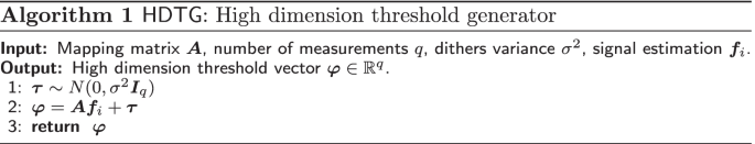
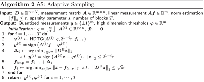
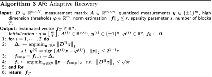
In this section, we present the general procedure of our adaptive scheme in details. Our system model is built upon the optimization problem (4). A major part of this problem is to choose an efficient threshold $\varvec{\varphi }\in {\mathbb {R}}^m$. To this end, we propose a closed-loop feedback system (see Fig. 1) which exploits prior information from previous stages. The superscript (i) corresponding to an element represents the i-th stage of that element in the adaptive algorithm. Our adaptive approach consists of three algorithms high-dimensional threshold generator (${\mathsf {HDTG}}$), adaptive sampling (${\mathsf {AS}}$) and adaptive recovery (${\mathsf {AR}}$). ${\mathsf {HDTG}}$ specifies the method of choosing the thresholds based on previous estimates. ${\mathsf {AS}}$ takes one-bit measurements of the signal by using ${\mathsf {HDTG}}$ and returns the one-bit samples and corresponding thresholds. Lastly, ${\mathsf {AR}}$ recovers the signal given the one-bit measurements. We provide a mathematical framework to guarantee our algorithm results in the following.

Theorem 1

(Main theorem) Let $r,c_{\epsilon },\gamma ,\epsilon >0$. Consider $\varvec{f}\in {\mathbb {R}}^n$ as the desired effective s-analysis-sparse signal with $\Vert \varvec{f}\Vert _2\le r$ and $\varvec{A}\in {\mathbb {R}}^{m\times n}$ is the measurement matrix with standard normal entries where m is the total number of measurements divided into T stages. Assume that

$$\begin{aligned}{}[\varvec{y}, \varvec{\varphi }]& = {\mathsf {AS}}(\varvec{A},\varvec{f},\varvec{D},r,T), \end{aligned}$$

(5)

$$\begin{aligned} \varvec{f}_{T}&= {\mathsf {AR}}(\varvec{A},\varvec{D}, \varvec{y}, \varvec{\varphi }, r,T) \end{aligned}$$

(6)

be the sampling and recovery algorithms introduced later in Algorithms 2 and 3, respectively, where $\varvec{\varphi }$ is determined by Algorithm 1. Then, with probability at least $1- \gamma \exp (\tfrac{-c_{\epsilon }m}{T})$ over the choice of $\varvec{\varphi }$ and $\varvec{A}$, the output of Algorithm 3 satisfies

$$\begin{aligned} \Vert \varvec{f}-\varvec{f}_{T}\Vert _{2}\le \epsilon r2^{1-T}. \end{aligned}$$

(7)

Proof

See Appendix 5.1. $\square$

A remarkable note is that if we only consider one stage, i.e., $T=1$, the exponential behavior of our error bound disappears and reaches the state-of-the-art error bound [8, Theorem 8]. In fact, the results of [8] are a special case of our work when the thresholds are non-adaptive. The term adaptivity is related to the threshold updating, and the measurement matrix ($\varvec{A}$) is fixed.

In what follows, we provide rigorous explanations about our proposed algorithms 1, 2 and 3 in three items.

• 1. High-Dimensional Threshold: Our algorithm for high-dimensional threshold selection is given in Algorithm 1. The algorithm output consists of two parts: deterministic (i.e., $\varvec{A}\varvec{f}_{i}$) and random (i.e., $\varvec{\tau }\in {\mathbb {R}}^q$) . The former transfers the origin to the previous signal estimate ($\varvec{f}_{i}$), while the latter creates measurement dithers from the origin. (The variance parameter $\sigma ^2$ controls the threshold distance from $\varvec{f}_{i}.$)

  

• 2. Adaptive Sampling: Our adaptive sampling algorithm is given in Algorithm 2. To implement this algorithm, we need the dictionary $\varvec{D}\in {\mathbb {R}}^{n\times N}$, the measurement matrix $\varvec{A}\in {\mathbb {R}}^{m\times n}$, linear measurement $\varvec{A}\varvec{f}$ and an over estimation of signal power r ($\left\| \varvec{f}\right\| _{2}\le r$). At the first stage, we initialize signal estimation to zero vector. We choose T stages for our algorithm. At the i-th stage, the measurement matrix $\varvec{A}^{(i)}$ is taken from the i-th row subset (of size $q:=\left\lfloor {\tfrac{m}{T}}\right\rfloor$) of $\varvec{A}$. The adaptive sampling process consists of four essential parts. First, in step 2 of the pseudocode, we generate the high-dimensional thresholds using Algorithm 1 by the parameters $\sigma ^2=2^{1-i}r$ and $\varvec{f}_i$. Second, we compare the linear measurement block $\varvec{A}^{(i)}\varvec{f}$ with the threshold vector $\varvec{\varphi }^{(i)}$ and obtain the sample vector $\varvec{y}^{(i)}$ (step 3 of Algorithm 2). Third, we implement a second-order cone program (steps 4 and 5) to find an approximate for $\varvec{f}$. However, this strategy does not often lead to an effective dictionary-sparse signal. So, in step 6, we devise a strategy to find a low-complexity approximation of $\varvec{f}$ with respect to operator $\varvec{D}^{\mathrm{H}}$. In other words, we project the resulting signal onto the nearest effective s-analysis-sparse signal. We refer to the third part of the adaptive sampling algorithm (steps 4–6) as single-step recovery (SSR). The estimated signal at each stage ($\varvec{f}_{i}$) builds the deterministic part of our high-dimensional threshold in step 2. Finally, Algorithm 2 returns binary vectors $\{\varvec{y}^{(i)}\}_{i=1}^T$ and the threshold vectors $\{\varvec{\varphi }^{(i)}\}_{i=1}^T$ to the output.

  

  

• 3. Adaptive Recovery: In the recovery procedure (Algorithm 3), we need the dictionary $\varvec{D}$, the measurement matrix $\varvec{A}$, binary measurements vector $\varvec{y}$, high-dimensional threshold vector $\varvec{\varphi }$ and an upper norm estimation of signal r. In the adaptive recovery algorithm, we first divide the inputs ($\varvec{y}$ and $\varvec{A}$) into T blocks (i.e., $\varvec{y}^{(i)}$ and $\varvec{A}^{(i)}$). Then, we simply implement SSR on each block. The output of SSR in the last stage is the final recovered signal (i.e., $\varvec{f}_T$).

2.1 Intuitive description of our algorithms

We provide here an example to clarify how our algorithm works. In this example, we consider a 2D point denoted by point DS (Fig. 2a) as the desired signal and depict the algorithm procedure for two consecutive iterations. At the first iteration of the algorithm, we do not have any estimation of the desired signal. Therefore, we set the first estimate to zero (equivalently $[0,0,1]^T$ in the 3D domain or point P in Fig. 2a). We generate high-dimensional thresholds and take four measurements (step 2 of $\mathsf {AS}$). These measurements are equivalently four hyperplane crossing the center of the hemisphere (Fig. 2b, step 3 of $\mathsf {AS}$). In the next step, we implement the augmented random hyperplane tessellation on the hemisphere and compute the first estimate of the desired signal and project it to the signal domain (steps 3–6 of $\mathsf {AS}$). In this example, we consider the point B as the first estimate ($\varvec{f}_{1}$ in first iteration of $\mathsf {AS}$). In the next iteration, we transfer the hemisphere to the adjacent point B and reduce the radius by a factor of two (Fig. 2c). The point B is the high-dimensional threshold of the second iteration of the algorithm. We perform our algorithm with four measurements. The main advantage of the reduction in the radius of the hemisphere (equivalently the variance argument of the threshold generator) is to get more precise measurements in the neighborhood of the desired signal. In the second stage of the algorithm, we take measurements (or equivalently hyperplanes) around the threshold, leading to locate measurements more concentrated around the desired signal. The intersection of hyperplanes and signal space in this example creates a new feasible set border which is depicted by the red line in Fig. 2d. In this intuitive description, we tried to clarify the random hyperplane tessellation usage in our proof sketch.⁴.

Fig. 2

3D illustration of random hyperplane tessellation for the first example of intuitive description

In the second example, we follow our algorithm steps in a 2D example and compare it with the non-adaptive algorithm. In Fig. 3a, we perform the non-adaptive algorithm for eight measurements. It is obvious that the solid lines ($L_5 - L_8$) or equivalently measurements do not have any impact on the final result. However, if we get these measurements in two iterations (i.e., stages) of the adaptive algorithm, the second bunch of samples ($L_5 - L_8$ in Fig. 3(b)) is more concentrated toward the desired signal ($\varvec{f})$.

Fig. 3

This figure compares the sampling procedure of the non-adaptive algorithm (a) with our adaptive algorithm (b)

3 Experimental results and discussion

In this section, we investigate the performance of our algorithm and compare it with the two previous one-bit dictionary-sparse recovery given by [8]. The first algorithm solves linear programming optimization (LP) [8, Subsection  4.1], and the second algorithm solves a second-order cone programming (CP) optimization [8, Subsection  4.2]. First, we construct a matrix where its columns are drawn randomly and independently from ${\mathbb {S}}^{n-1}$. Then, the dictionary $\varvec{D}\in {\mathbb {R}}^{n\times N}$ ($N=1000,n=50$) is defined as an orthonormal basis of this matrix. Then, the signal $\varvec{f}$ is generated as $\varvec{f}=\varvec{B}\varvec{c}$ where $\varvec{B}$ is a basis of ${\mathrm{null}}(\varvec{D}_{\overline{{\mathcal {S}}}})$ and $\varvec{c}$ is drawn from standard normal distribution. Here, $\overline{{\mathcal {S}}}$ is used to denote the complement of the support of $\varvec{D}^{\mathrm{H}}\varvec{f}$. The elements of $\varvec{A}$ are chosen from i.i.d. standard normal distribution. We set $r= 2\Vert \varvec{f}\Vert _{2}$, $\sigma =r$ and the number of stages to $T=10$. Define the normalized reconstruction error as $\tfrac{\Vert \varvec{f}-\hat{\varvec{f}}\Vert _{2}}{\Vert \varvec{f}\Vert _{2}}$ ($\hat{\varvec{f}}$ denotes the estimated signal in each algorithm, and it is represented by $\varvec{f}_{T}$) especially in our algorithm. The results in Fig. 4a are obtained by implementing Algorithms 2 and 3 100 times and taking the average of the normalized reconstruction error. As it is clear from Fig. 4a, LP algorithm outperforms CP by 2 dB on average. Our algorithm with few measurements behaves slightly weaker than others. The proposed approach requires a minimum number of measurements to act perfectly. The main reason for this behavior is our thresholding scheme. The variance of dithers is reduced in each iteration (i.e., stage). We also take the measurements around the previous estimate of the desired signal. On the contrary, the CP and LP algorithms only reduce the signal space uniformly. When the number of measurements is below the required bound, our first estimate gets away from the desired signal, so the adaptive algorithm tries to find it around a false estimate. However, it seems that there is a phase transition behavior in our algorithm when the number of measurements increases. In fact, after a certain number of measurements, our proposed algorithm substantially outperforms both LP and CP. Table 1 shows the average execution time (CPU time) of the three algorithms per the specified number of measurements.

Table 1 Average execution time (millisecond)

In the second experiment, we examine the performance of our algorithm for multiple degrees of sparsity. Figure 4b shows the result for $s = 20, 30, 40.$ (Other parameters are assumed similar to the first experiment.) As it is clear from the figure, by increasing the sparsity level, the accuracy is decreased.

Fig. 4

Reconstruction of a dictionary-sparse signal $\varvec{x}\in {\mathbb {R}}^{50}$ in the dictionary $\varvec{D}\in {\mathbb {R}}^{50\times 1000}$. Both figures show the reconstruction error averaged over 100 Monte Carlo simulations. Image a compares the performance of the algorithms in $s=20$. Image b examines the performance of our algorithm over different sparsity levels

In the third experiment, we consider the Shepp–Logan phantom image as the ground-truth signal. Since the required number of measurements in one-bit CS is significantly larger than that of the conventional CS (see, e.g., [13, Section 5]), we split the picture into multiple blocks of size $32\times 32$ and process each block separately, merely due to computational complexity reasons. This block processing allows us to implement the algorithm in multiple threads and reduce the execution time. We use a redundant wavelet dictionary and $10^5$ Gaussian measurements to recover each block. We evaluate the reconstruction quality of final result in terms of the peak signal-to-noise ratio (PSNR) given by

$$\begin{aligned} {\text {PSNR}}\left( \varvec{X},\widehat{\varvec{X}}\right) = 20 \log _{10}\left( \tfrac{\Vert \varvec{X}\Vert _{\infty }256}{\Vert \varvec{X}-\widehat{\varvec{X}}\Vert _{F}}\right) , \end{aligned}$$

(8)

where $\varvec{X}$ and $\widehat{\varvec{X}}$ are the true and estimated images. As shown in Fig. 5, LP (Fig. 5b) and CP (Fig. 5c) algorithms clearly fail with poor performances, but as it is evident in Fig. 5d, the output of our algorithm is almost similar to the desired picture.

Fig. 5

Simulation results for reconstruction of the Shepp–Logan phantom image (phantom(256) in MATLAB) in which the picture split to $32 \times 32$ blocks and each algorithm get $m=10^5$ measurements per block

4 Conclusion

This paper proposed a one-bit compressed sensing algorithm that recovers dictionary-sparse signals from binary measurements by adaptively exploiting the inherent information in the sampling procedure. This scheme helps to reduce the number of needed measurements substantially. In addition, our algorithm exhibits an exponential decaying behavior in the reconstruction error. The proof approach is based on geometric theories in the high-dimensional estimation. In this work, we used geometric intuition to explain our result, which also can be used in other areas of signal processing. We believe our analysis can be extended to the multi-bit setting. We used a fixed reduction pattern in the thresholds dithers throughout this work. We believe that this reduction can be chosen smartly by extracting the geometric features in each algorithm step.

5 Proofs

5.1 Proof of Theorem 1

Proof

By induction law, we show that

$$\begin{aligned} \Vert \varvec{f}-\varvec{f}_{i}\Vert _{2}\le \epsilon r2^{1-i} \end{aligned}$$

(9)

holds with high probability for any $i\in \{1,\dots ,T\}$. Consider the first step, i.e., $i=1$ in Algorithm 2. At this step, our initial estimate $\varvec{f}_0$ is equal to $\varvec{0}$. Thus, the output of Algorithm 1 only contains the random part of high-dimensional thresholds (step 2 of Algorithm 2). Then, we obtain $\varvec{f}_1$ by using steps 4–9 of Algorithm 2 (except that we assume $\sigma =r$ in Algorithm 2 and $q = \left\lfloor {\tfrac{m}{T}}\right\rfloor$). As a result, to verify $\Vert \varvec{f}-\varvec{f}_{1}\Vert _{2}\le \epsilon r$, we use [8, Theorem 8] to prove our result: $\square$

Theorem 2

[8, Theorem 8] Let $\epsilon ,r,\sigma >0$, let

$$\begin{aligned} m \ge C \left( \tfrac{r}{\sigma } +\tfrac{\sigma }{r} \right) ^{-6}\left( \tfrac{r^{2}}{\sigma ^{2}}+1\right) \epsilon ^{-6} s \ln (\tfrac{eN}{s}) \end{aligned},$$

and let $\varvec{A}\in {\mathbb {R}}^{m\times n}$ be populated by independent standard normal random variables. Furthermore, let $\tau _{1}, \ldots , \tau _{m}$ be independent normal random variables with mean zero and variance $\sigma ^{2}$ that are also independent from $\varvec{A}$. Then, with failure probability at most $\gamma \exp (\tfrac{-c^{\prime }m \epsilon ^{2}r^{2}\sigma ^{2}}{(r^{2}+\sigma ^{2})^{2}})$, any signal $\varvec{f}\in {\mathbb {R}}$ with $\Vert \varvec{f}\Vert _{2} \le r$, $\Vert \varvec{D}^{\mathrm{H}}\varvec{f}\Vert _{1} \le \sqrt{s} r$ and observed via $\varvec{y}= {\text {sign}}(\varvec{A}\varvec{f}-\varvec{\tau })$ is approximated by

$$\begin{aligned} \varvec{f}_{\mathrm{{CP}}}=\mathop {\arg \min }_{\varvec{z}\in {\mathbb {R}}^{n}} ~ \left\| \varvec{D}^{\mathrm{H}}\varvec{z}\right\| _{1} ~{\text {s.t.}}~ \varvec{y}= {\mathrm{sign}}(\varvec{A}\varvec{z}-\varvec{\tau }),~ \Vert \varvec{z}\Vert _{2}\le r, \end{aligned}$$

with error

$$\begin{aligned} \Vert \varvec{f}-\varvec{f}_{\mathrm{{CP}}}\Vert _{2}\le \epsilon r. \end{aligned}$$

(10)

Now, suppose that the result (9) holds in the $(i-1)$-th step, i.e.,

$$\begin{aligned} \Vert \varvec{f}-\varvec{f}_{i-1}\Vert _{2}\le \epsilon r2^{2-i}. \end{aligned}$$

(11)

Consider i-th stage of Algorithm 2 where the high-dimensional thresholds and the measurements are obtained as

$$\begin{aligned} \varvec{\varphi }^{\left( i\right) }\leftarrow {\mathsf {HDTG}}(\varvec{A}^{(i)},q,2^{1-i}r,\varvec{f}_{i-1}), \end{aligned}$$

(12)

$$\begin{aligned} \varvec{y}^{\left( i\right) } = {\text {sign}}\left( \varvec{A}^{(i)}\varvec{f}-\varvec{\varphi }^{\left( i\right) }\right) . \end{aligned}$$

(13)

By substituting (12) in (13), we reach:

$$\begin{aligned} \varvec{y}^{\left( i\right) } = {\text {sign}}\left( \varvec{A}^{(i)}(\varvec{f}-\varvec{f}_{i-1})-\varvec{\tau }^{(i)}\right) . \end{aligned}$$

(14)

Since $\varvec{f}$ is effective s-analysis-sparse with $\Vert \varvec{f}\Vert _2\le 1$, we have that $\Vert \varvec{D}^H\varvec{f}\Vert _1\le \sqrt{s}\Vert \varvec{f}\Vert _2$. Further, the output of Algorithm 2 at the $(i-1)$-th stage satisfies, i.e., $\Vert \varvec{D}^H\varvec{f}_{i-1}\Vert _1\le \sqrt{s}r$, and it then holds that the signal $\varvec{f}-\varvec{f}_{i-1}$ satisfies $\Vert \varvec{D}^H(\varvec{f}-\varvec{f}_{i-1})\Vert _1\le \Vert \varvec{D}^H\varvec{f}\Vert _1+\Vert \varvec{D}^H\varvec{f}_{i-1}\Vert _1\le 2\sqrt{s} r=\sqrt{2^{2i-2} \epsilon ^{-2} s} \epsilon 2^{-i}r:=\sqrt{s'}r'$. Now, by leveraging the assumption in (11), we can directly apply Theorem 2 to this signal. In simple words, we set

$$\begin{aligned}&{\varvec{f}}\leftarrow {\varvec{f}}-{\varvec{f}}_{i-1}, \\&r\leftarrow \epsilon 2^{2-i}r, \\&\sigma \leftarrow \epsilon 2^{2-i}r, \\&s\leftarrow s^{\prime}. \end{aligned}$$

(15)

in Theorem 2. As a result, by exploiting this theorem and some simplifications, we shall have that

$$\begin{aligned} \left\| \varvec{f}-\varvec{f}_{i-1}-\varvec{\Delta }_{i}\right\| _{2} \le \epsilon _1 r':= \epsilon r 2^{-i}, \end{aligned}$$

(16)

with probability at least $1- \gamma \exp (-c^{\prime }_{\epsilon } q)$ where in the latter expression we used $\epsilon _1=\frac{1}{4}$ and $\varvec{\Delta }_i$ is the output vector of the optimization problem in step 4 of Algorithm 2. $c^{\prime }_{\epsilon }$ is a certain constant dependent on $\epsilon$. Now, suppose that (16) occurs. Consider

$$\begin{aligned} \varvec{f}_{\mathrm{tmp}}=\varvec{f}_{i-1}+\varvec{\Delta }_{i}. \end{aligned}$$

(17)

After applying step 6 of Algorithm 2, we obtain $\varvec{f}_i$ that has the property

$$\begin{aligned} \Vert \varvec{D}^{\mathrm{H}}\varvec{f}_i\Vert _1\le \sqrt{s}r. \end{aligned}$$

Then, we have

$$\begin{aligned} \Vert \varvec{f}-\varvec{f}_i\Vert _2\le \Vert \varvec{f}-\varvec{f}_{\mathrm{tmp}}\Vert _2+\Vert \varvec{f}_{\mathrm{tmp}}-\varvec{f}_i\Vert _2. \end{aligned}$$

(18)

Finally, by using (16), (17), and the fact that $\Vert \varvec{f}_i-\varvec{f}_{\mathrm{tmp}}\Vert _2\le \Vert \varvec{f}-\varvec{f}_{\mathrm{tmp}}\Vert _2$ (step 6), the latter equation becomes

$$\begin{aligned} \Vert \varvec{f}-\varvec{f}_i\Vert _2\le \epsilon 2^{1-i}r \end{aligned}$$

(19)

Since we consider T stage in Algorithms 2 and 3, we reach the error bound:

$$\begin{aligned} \left\| \varvec{f}-\varvec{f}_{T}\right\| _{2} \le \epsilon r 2^{1-T}. \end{aligned}$$

(20)

References

D.L. Donoho, Compressed sensing. IEEE Trans. Inf. Theory 52(4), 1289–1306 (2006)
E.J. Candès, et al., Compressive sampling, in Proceedings of the International Congress of Mathematicians, vol. 3, pp. 1433–1452 (2006). Madrid, Spain
P.T. Boufounos, R.G. Baraniuk, 1-bit compressive sensing, in 2008 42nd Annual Conference on Information Sciences and Systems, pp. 16–21 (2008). IEEE
E.J. Candès, Y.C. Eldar, D. Needell, P. Randall, Compressed sensing with coherent and redundant dictionaries. Appl. Comput. Harmon. Anal. 31(1), 59–73 (2011)
M. Genzel, G. Kutyniok, M. März, l1-analysis minimization and generalized (co-) sparsity: when does recovery succeed? Appl. Comput. Harmon. Anal. 52, 82–140 (2021)
S. Daei, F. Haddadi, A. Amini, M. Lotz, On the error in phase transition computations for compressed sensing. IEEE Trans. Inf. Theory 65(10), 6620–6632 (2019)
S. Daei, F. Haddadi, A. Amini, Living near the edge: a lower-bound on the phase transition of total variation minimization. IEEE Trans. Inf. Theory 66(5), 3261–3267 (2019)
R. Baraniuk, S. Foucart, D. Needell, Y. Plan, M. Wootters, One-bit compressive sensing of dictionary-sparse signals. Inf. Inference J. IMA 7(1), 83–104 (2018)
A. Zymnis, S. Boyd, E. Candes, Compressed sensing with quantized measurements. IEEE Signal Process. Lett. 17(2), 149–152 (2010)
L. Jacques, J.N. Laska, P.T. Boufounos, R.G. Baraniuk, Robust 1-bit compressive sensing via binary stable embeddings of sparse vectors. IEEE Trans. Inf. Theory 59(4), 2082–2102 (2013)
Y. Plan, R. Vershynin, One-bit compressed sensing by linear programming. Commun. Pure Appl. Math. 66(8), 1275–1297 (2013)
U.S. Kamilov, A. Bourquard, A. Amini, M. Unser, One-bit measurements with adaptive thresholds. IEEE Signal Process. Lett. 19(10), 607–610 (2012)
R.G. Baraniuk, S. Foucart, D. Needell, Y. Plan, M. Wootters, Exponential decay of reconstruction error from binary measurements of sparse signals. IEEE Trans. Inf. Theory 63(6), 3368–3385 (2017)
K. Knudson, R. Saab, R. Ward, One-bit compressive sensing with norm estimation. IEEE Trans. Inf. Theory 62(5), 2748–2758 (2016)
F. Wang, J. Fang, H. Li, Z. Chen, S. Li, One-bit quantization design and channel estimation for massive mimo systems. IEEE Trans. Veh. Technol. 67(11), 10921–10934 (2018)
Funding
There is no funding for the research of this paper.
Author information
Authors and Affiliations