Theoretical formulation/development of signal sampling with an equal arc length using the frame theorem

Abstract

Nonuniform sampling with equal arc length intervals can be found in shape measurements with contact sensor arrays. In this study, the conditions of nonuniform spatial sampling with an equal arc length interval are derived from two frame theorems. First, for general nonuniform sampling, the condition is that the equal arc length interval of the sensors should be less than $\frac{1}{4\Omega }$. Second, for strictly increasing sampling (the sampling point set is strictly increasing), the condition is that the equal arc length interval of the sensors should be less than $\frac{1}{2\Omega }$. The $\Omega$ is the maximum frequency of the detected object. For the latter, if the sampling frequency is more than twice the sampling frequency required, the reconstruction error (RRMSE and MRE) is less than 5%. If the sampling frequency is more than 2.5 times, the reconstruction error is less than 3%. The simulation and the application test are carried out, and the results show that a sensor array with equal arc length interval can reconstruct the detected object with high accuracy.

1 Introduction

Sampling plays a critical role in signal analysis and contact sensor shape detection. However, samples cannot be collected uniformly in various applications, such as underwater terrain subsidence monitoring based on a MEMS 9-axis sensor array [1,2,3], shape monitoring based on the fiber Bragg grating (FBG) sensor array [4,5,6,7,8,9,10], and data gloves or motion capture devices based on fiber curvature sensor arrays [11, 12]. The sensor array has an implicit characteristic—the arc length interval between the sensors is equal and constant when the sensor array moves with the detected object. Therefore, the sampling of the sensor array becomes nonuniform even though the sensor array is deployed in an equal arc interval at the beginning (uniform sampling at the beginning) when the sensor array moves with the detected object.

Whether the detected object can be completely reconstructed from its nonuniform spatial sampled values with the condition of equal arc interval is a general and important problem which should be studied. There are two reasons: One is that it cannot be sure if the reconstructed signal is not distorted from the nonuniform sampling set obtained from the contact sensor array. The other is that more sensors are often used to ensure the reconstruction without distortion, resulting in increased costs, more complex systems and larger data volumes if the nonuniform sampling conditions are not known.

Consequently, there have been studies on randomized nonuniform sampling [13,14,15,16,17,18] and periodic nonuniform sampling [19,20,21,22]. For randomized nonuniform sampling, the nonuniform samples are often regarded as random perturbations from a uniform sampling grid in the analysis [17]. The nonuniform sampling set has random characters. The sampling times are often constructed by adding a Gaussian distribution sampling noise to the previous sampling time. Xu et al. [17] considered the second-order random statistic characters; the randomized nonuniform sampling is equivalent to the uniform sampling of the signal after a pre-filter. The pre-filter is a fractional multiplicative filter. The reference [23] derived the sampling methods for random signals with known spectral densities in the mean square sense, including uniform and nonuniform sampling. The sampling theorem in the fractional Fourier domain and its relation to the von Neumann ergodic theorem were also discussed in [24].

For periodic nonuniform sampling, the offset of sampling time $t_{n}$ from the equal interval sampling time sequence nT has a periodic structure with a period of M, where T is the average sampling period and M is an integer. The sampling time is $t_{n} = nT + r_{n} T = (kM + m)T + r_{m} T$, where $r_{n} T$ is the offset of $t_{n}$ from nT and $m \equiv n\;(\bmod \;M)$ [22]. This means that the adjacent sampling points are not uniform, but the interval between each sampling point and the subsequent sampling point is equal. The total sampling period is MT [25, 26]. It is often applied in analog-to-digital (A/D) sampling technology, combining M AD converters with lower sampling rate to obtain one virtual sensor with high sampling rate [22]. Tao et al. [27] derived the periodic nonuniform sampling and reconstruction in the fractional Fourier domain. The sampling theorem verified that if a signal was band-limited or compact in a fractional Fourier domain, it could be sampled by using the fractional Fourier transform instead of the Fourier transform with a larger sampling interval. The fractional Fourier Transform has been proved as a perfect tool to improve the reconstruction quality [28].

However, nonuniform sampling with the condition of equal arc interval is neither the randomized nonuniform sampling with a known distribution such as Gaussian distribution sampling noise nor periodic nonuniform sampling. There is no research on nonuniform spatial sampling for contact sensor arrays with the condition of equal arc interval. In this article, two theorems of nonuniform spatial sampling with the condition of equal arc interval are studied. The definition of nonuniform spatial sampling and associated mathematical expression are given. Then, the condition of nonuniform spatial sampling is derived from the frame theorem. For general nonuniform spatial sampling, the condition of sampling interval is obtained by the Kadec theorem. For the strictly increasing sampling set, the condition of sampling interval is obtained by the Benedetto theorem. In order to verify the correctness of the condition of nonuniform spatial sampling, two simulations and a test are carried out. Finally, a conclusion is presented.

2 Methods

2.1 Definition of nonuniform spatial sampling with the condition of equal arc interval

Figures 1 and 2 show uniform and nonuniform spatial sampling, respectively. The ‘o’ in Figs. 1 and 2 is the sampling point. In the uniform sampling, the interval of the x-axis is spaced equally, which is x in Fig. 1. In the nonuniform case, the interval of the x-axis is spaced unequally which is $(x_{i} { - }x_{i - 1} ) \ne (x_{i + 1} { - }x_{i} ),i = 1,2,3 \ldots$ (Fig. 2) and the arc length of $,i \ne j$ is equal. The sampling point set $\left\{ {x_{i} ,i = 0,1,2,3 \ldots } \right\}$ is strictly increasing when $x_{i} { - }x_{i - 1} > 0$ for any i.

Fig. 1

Uniform spatial sampling

Fig. 2

Nonuniform spatial sampling

2.2 The mathematical expression of the nonuniform spatial sampling with the condition of equal arc interval

Assume that $f(x),x \in \left[ {0,L} \right]$ is a mathematical expression of a detected object (such as a ribbon of terrain) which is a band-limited function. The terrain is detected by a MEMS 9-axis sensor array [1,2,3]. In other words, $f(x)$ is sampled with the condition of equal arc length. N is the sample number which can be obtained by $N = {L \mathord{\left/ {\vphantom {L X}} \right. \kern-\nulldelimiterspace} X}$ (L is the arc length of the $f(x)$, and x is the arc length of sensors which have an equal spatial interval at the beginning). Set $f_{s} (x) = f(x_{n} )$ is the sampling value. Like the process of uniform sampling, nonuniform sampling is the product of a series of impulse series and the original function.

Figure 3 shows the process of nonuniform spatial sampling with equal arc length. In contrast to uniform sampling, the impulse series does not have periodicity (equal intervals), which can be expressed as

$$S\left( {x_{n} } \right) = \sum\limits_{n = 1}^{N} {\delta (x - x_{n} )}$$

(1)

where $x_{n}$ is the projection of the sampling point on the x-axis. Sampled signal $f_{s} (x)$ is the product of the impulse series $S\left( {x_{n} } \right)$ and the original function $f(x)$, which shows as

$$\begin{aligned} f_{s} (x) = & f(x) \cdot S(x_{n} ) \\ = & \sum\limits_{n = 1}^{N} {f(x_{n} ) \cdot \delta (x - x_{n} )} \\ \end{aligned}$$

(2)

As seen from formula (2), the sampled signal $f_{s} (x)$ is an impulse series weighted by the values $f(x_{n} )$.

Fig. 3

Process of the nonuniform sampling

2.3 The condition of nonuniform sampling with equal arc length

2.3.1 Frame theorem

A sequence $\{ f_{n} ,n \in {\mathbf{\mathbb{Z}}}\}$ in a Hilbert space ${\rm H}$ is called a frame [17, 29, 30], if there exist constants $A,B > 0$, such that for all $f \in H$,

$$A\left\| f \right\|^{2} \le \sum\limits_{{n \in {\mathbf{\mathbb{Z}}}}} {\left| {\left\langle {f,f_{n} } \right\rangle } \right|}^{2} \le B\left\| f \right\|^{2}$$

(3)

where $\langle \; \rangle$ is the inner product, which is defined as $\left\langle {f,f_{n} } \right\rangle = \int\limits_{\mathbb{R}} {f(x)\overline{{f_{n} (x)}} } dx$ ($\overline{{f_{n} (x)}}$ is the conjugation of $f_{n} (x)$, $\left\| f \right\|$ is the norm of the f which is $\left\| f \right\| = \left\langle {f,f} \right\rangle^{\frac{1}{2}}$.

In the frame theorem, the sampling point set is $\{ x_{n} \}_{{n \in {\mathbb{Z}}}}$ and the sampling value set is $\{ f(x_{n} )\}_{{n \in {\mathbb{Z}}}}$. In order to completely reconstruct the band-limited function $f(x)$ from the sampling value set $\{ f(x_{n} )\}_{{n \in {\mathbb{Z}}}}$, the following inequality (4) should be met.

$$A\left\| f \right\|^{2} \le \sum\limits_{n \in Z} {\left| {f(x_{n} )} \right|}^{2} \le B\left\| f \right\|^{2}$$

(4)

where $f(x) \in PW_{\Omega }$,which is the Paley–Wiener space. It is defined as $PW_{\Omega } = \left\{ {f(x) \in L^{2} ({\mathbb{R}}):{\text{supp}} \hat{f} \subseteq [ - \Omega ,\Omega ]} \right\}$. It is a Hilbert space, considered as a closed subspace of $L^{2} ({\mathbb{R}})$ taken with the $L^{2}$-norm. $\hat{f}$ is the Fourier transform of the $f(x)$.$\hat{f}(\xi ) = \mathop {\lim }\limits_{n \to \infty } \int\limits_{ - n}^{n} {f(x)e^{ - 2\pi i\xi x} dx}$. The support condition, ${\text{supp}} \hat{f} \subseteq [ - \Omega ,\Omega ]$, is described by saying that f is $\Omega$-band-limited. $\hat{f}(\xi ) = 0$ when $\left| \xi \right| \ge \Omega$. $\Omega$ is the maximum frequency of function $f(x)$. When $\{ e^{{j2\pi \Omega x_{n} }} \}_{{n \in {\mathbb{Z}}}}$ is the frame for $PW_{\Omega }$, the function $f(x)$ can be reconstructed by the sampling value set $\{ f(x_{n} )\}_{{n \in {\mathbb{Z}}}}$.

2.3.2 Condition of nonuniform sampling with equal arc length

• (1) The general nonuniform sampling with equal arc length.

  From the Kadec theorem [3], when the sampling point set $\{ x_{n} \}_{{n \in {\mathbb{Z}}}}$ satisfies inequality (5)

  $$\mathop {{\text{sup}}}\limits_{n \in Z} \left| {x_{n} - \frac{n}{2\Omega }} \right| < \frac{1}{4} \times \frac{1}{2\Omega },$$

  (5)

  $\{ e^{{j2\pi \Omega x_{n} }} \}_{{n \in {\mathbb{Z}}}}$ is the frame of $PW_{\Omega }$. Inequality (5) can be expanded as

  $$- \frac{1}{4} \times \frac{1}{2\Omega } < x_{n} - \frac{n}{2\Omega } < \frac{1}{4} \times \frac{1}{2\Omega }$$

  (6)

  Then, inequality (6) can be expressed as

  $$- \frac{1}{8\Omega } + \frac{n}{2\Omega } < x_{n} < \frac{1}{8\Omega } + \frac{n}{2\Omega }$$

  (7)

  From inequality (7), it can be concluded that when the spatial arc length interval of the sensor array is not greater than $\frac{1}{4\Omega }$, there is more than one sampling point in the range $\left[ {(n - 1)\frac{1}{4\Omega },n\frac{1}{4\Omega }} \right],n = 1,2, \ldots$, and the sampling point set is denoted as $\{ x_{n} \}$. Then, values can be extracted from the set $\{ x_{n} \}$ and form a new set $\{ \tilde{x}_{n} \}$ which should satisfy the inequality (7). The derivation process is as follows: Fig. 4 shows the derivation schematic diagram of the spatial sampling interval. Taking n = 1 for example, assume that there is a sampling point in the range $\left[ {\frac{1}{4\Omega },\frac{1}{2\Omega }} \right]$. When the sampling point is in the range $\left[ {\frac{3}{8\Omega },\frac{1}{2\Omega }} \right]$ (dash area in Fig. 4), inequality (7) is satisfied. When the sampling point is in the range $\left[ {\frac{1}{4\Omega },\frac{3}{8\Omega }} \right]$ (blue area in Fig. 4), there must be another sampling point in the range $\left[ {\frac{3}{8\Omega },\frac{5}{8\Omega }} \right]$(yellow area in Fig. 4), satisfying inequality (7). This is because the interval of the range $\left[ {\frac{3}{8\Omega },\frac{5}{8\Omega }} \right]$ and maximum spatial interval is equal, which is $\frac{1}{4\Omega }$. Moreover, when there is more than one sampling point in the range $\left[ {\frac{1}{4\Omega },\frac{1}{2\Omega }} \right]$, the derivation above is also set up. Therefore, a new set $\{ \tilde{x}_{n} ,n = 1,2, \ldots ,N\}$ always can be extracted which satisfies inequality (7). In other words, when the arc length interval of the sensor array is not greater than $\frac{1}{4\Omega }$, inequality (5) is satisfied. The frame bound A and B are not given in inequality (4). It is given by theorem 1.

  Fig. 4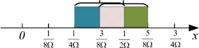

  

  Derivation schematic diagram of the spatial sampling interval

  Theorem 1

  [3]: Assume that there are constant $\varepsilon$, $\alpha$ and $\beta$, $0 < \varepsilon < 1$, $\alpha > 0$, $\beta > 0$, and sampling point set $\{ x_{n} \}_{{n \in {\mathbb{Z}}}}$ satisfied the following two inequalities, denoted as condition 2 and condition 3, respectively:

  $$\left\{ {\begin{array}{*{20}c} {\left| {x_{n} - x_{m} } \right| \ge \alpha > 0, \, n \ne m} \\ {\mathop {{\text{sup}}}\limits_{n \in Z} \left| {x_{n} - \varepsilon \frac{n}{2\Omega }} \right| \le \beta < \infty } \\ \end{array} } \right.$$

  (8)

  Then, there exist constants A and B, $0 < A \le B$, that are related to $\varepsilon$, $\alpha$ and $\beta$ such that inequality (4) for all $f \in PW_{\Omega }$.

  Derivation of sampling conditions: The sampling point set $\{ x_{n} \}_{{n \in {\mathbb{Z}}}}$ satisfies condition 2, $\left| {x_{n} - x_{m} } \right| \ge \alpha > 0$, when the detected object is not vertical (actually, the case of vertical is similar to the horizontal case). In other words, the spatial sampling interval between sampling points always is greater than zero, and there exists $\alpha$, which satisfies condition 2, $\left| {x_{n} - x_{m} } \right| \ge \alpha > 0$.

  For condition 3, $\mathop {{\text{sup}}}\limits_{n \in Z} \left| {x_{n} - \varepsilon \frac{n}{2\Omega }} \right| \le \beta < \infty$ can be interpreted that all sampling points $x_{n}$ need to satisfy $- \beta \le x_{n} - \varepsilon \frac{n}{2\Omega } \le \beta$, which can be transformed as:

  $$- \beta + \varepsilon \frac{n}{2\Omega } \le x_{n} \le \beta + \varepsilon \frac{n}{2\Omega }$$

  (9)

  As the above analysis shows, there must exist a sampling point in the range $\left[ {(n - 1)\frac{1}{4\Omega },n\frac{1}{4\Omega }} \right],n = 1,2, \ldots ,2N$, which means that $(n - 1)\frac{1}{4\Omega } \le x_{n} \le n\frac{1}{4\Omega }$. Therefore, in order to satisfy inequality (9), inequality (10) should be satisfied:

  $$\left\{ {\begin{array}{*{20}l} {\frac{n}{4\Omega } \le \beta + \varepsilon \frac{n}{2\Omega }} \hfill \\ { - \beta + \varepsilon \frac{n}{2\Omega } \le \frac{n - 1}{{4\Omega }}} \hfill \\ \end{array} } \right.$$

  (10)

  Add the two inequalities in (10), then we get $\beta \ge \frac{1}{8\Omega }$. Set $\beta = \frac{1}{4\Omega }$ and use in the inequality $\frac{n}{4\Omega } \le \beta + \varepsilon \frac{n}{2\Omega }$ and simplifying, we get $\varepsilon \ge \frac{1}{4} - \frac{1}{n}$. What is more, $0 < \varepsilon < 1$, setting $\varepsilon = \frac{1}{4}\left( {n > 0} \right)$ is satisfied. Therefore, the sampling point set satisfies condition 2 and condition 3 at the same time when $\beta = \frac{1}{4\Omega }$ and $\varepsilon = \frac{1}{4}$.

  It can be seen that when the equal arc length interval between the sampling points is half of the Nyquist sampling interval or one quarter of the period corresponding to the highest frequency of the detected object, the original function $f(x)$ can be reconstructed completely. [End of derivation.]

  However, the sampling interval based on the nonuniform sampling theorem is larger. The more the sampling points, the more the sensors, the more complicated is the sensor network and the more cost. In applications such as underwater seabed monitoring based on sensors, the sampling point set is strictly increasing $\left\{ {x_{i} |x_{i} - x_{i - 1} > 0,i = 1,2,3 \ldots } \right\}$. Therefore, nonuniform sampling theorem for increasing sampling is introduced which can obtain a less sampling interval.

• (2) The nonuniform sampling of a strictly increasing sequence with equal arc length.

  Theorem 2

  In the frame theory, Marvasti [29] and Benedetto [30] state that the sample points set $\{ x_{n} ,n \in {\mathbb{R}}\} \subseteq {\mathbb{R}}$ are strictly increasing for which

  $$\mathop {\lim }\limits_{n \to \pm \infty } x_{n} = \pm \infty$$

  and

  $$0 < d \le \mathop {\inf }\limits_{n} (x_{n + 1} - x_{n} ) \le \mathop {\sup }\limits_{n} (x_{n + 1} - x_{n} ){ = }T < \infty$$

  For a given $\Omega > 0$, assume that $\Omega_{1} > \Omega$ satisfies the condition

  $$2T\Omega_{1} < 1$$

  Then, $\{ e^{{j2\pi \Omega x_{n} }} ,n \in {\mathbb{Z}}\}$ is a frame of $PW_{\Omega }$. Frame boundaries $A$ and $B$ satisfy inequalities $A \ge \frac{{(1 - 2T\Omega )^{2} }}{T}$ and $B \le \frac{4}{{\pi^{2} \Omega d^{2} }}(e^{\pi \Omega d} - 1)$. The frame of is exact, which means it is no longer a frame whenever anyone of its elements is removed.

  Derivation of sampling conditions: If the detected object is not a vertical line, such as the slope of detected terrain is less than 90°, the sampling point set $\{ x_{n} ,n = 1,2, \ldots ,N\}$ satisfies the condition of strict increase for all $x_{n}$. In practical applications, the detected object is limited, which means $\mathop {\lim }\limits_{n \to \pm \infty } x_{n} < \infty$. The sampling point set and sampling value set should be extended to satisfy the condition. The idea of extension is that for sampling points, the sampling points should strictly increase and the difference between adjacent sampling points is less than $\frac{1}{2\Omega }$. Therefore, the extension sampling point set $\{ \tilde{x}_{n} ,n = - \infty , \ldots ,1,2, \ldots ,\infty \}$ meets the condition of $\sup (\tilde{x}_{n + 1} - \tilde{x}_{n} ) < \frac{1}{2\Omega } < \infty$, $0 < \inf (\tilde{x}_{n + 1} - \tilde{x}_{n} )$ and $\mathop {\lim }\limits_{n \to \pm \infty } \tilde{x}_{n} = \pm \infty$. For the sampling values, the extended sample values are set as zeros and the original sample values were kept unchanged. Denote the extension sampling value set as $\{ f(\tilde{x}_{n} ),n = - \infty , \ldots ,1,2, \ldots ,\infty \}$; $f(\tilde{x}_{n} ) = 0$ was set when $n < 1$ and $n > N$. $f(\tilde{x}_{n} ) = f(x_{n} )$ was set when $n = 1,2, \ldots ,N$.

  It can be obtained that the nonuniform sampling set can completely reconstruct the original signal when the arc length interval of a sensor array is less than $\frac{1}{2\Omega }$, and there should be more than one sampling point in the range $\left[ {(n - 1)\frac{1}{2\Omega },n\frac{1}{2\Omega }} \right] = \left[ {(n - 1)\frac{\pi }{3},n\frac{\pi }{3}} \right],n = 1,2, \ldots ,N$. [End of derivation.]

  The main difference between the two frame theorems is whether the sampling point set satisfies strictly monotonically increasing. If not, it is a general nonuniform sampling; the sampling condition can be deduced that the equal arc length interval of the sensors should be less than $\frac{1}{4\Omega }$. If it does, it is a strictly increasing sampling, the condition is that the equal arc length interval of the sensors should be less than $\frac{1}{2\Omega }$. The $\Omega$ is the maximum frequency of the detected object. It is the minimum number of sampling points needed. It is proved theoretically that equal arc length nonuniform sampling can reconstruct the original signal, which can be used to guide technicians on the application of contact sensor arrays for shape monitoring.

3 Simulation

3.1 Simulation of general nonuniform spatial sampling theorem

A simulation for the nonuniform sampling condition and reconstruction method is carried out. Any signal can be superimposed by sinusoidal signals and cosine signals. Therefore, a cosine signal and a composite signal consisting of sine and cosine are selected for the simulation. The cosine signal is $f(x) = \cos (3x),x \in [0,10]$, and the composite signal is $f(x) = 0.5\sin (2x) + \cos (3x),x \in [0,10][0,10]$. According to reference [31], the sampling points are reconstructed by spline interpolation, which is used in this article.

The maximum frequency of both signals is $\Omega = \frac{3}{2\pi }$. According to the above analysis, the spatial sampling interval should be less than $\frac{1}{4\Omega } = \frac{\pi }{6} \approx 0.52$. The sampling interval is regarded as 0.5, and there must be more than one sampling point in the range $\left[ {(n - 1)\frac{1}{4\Omega },n\frac{1}{4\Omega }} \right] = \left[ {(n - 1)\frac{\pi }{6},n\frac{\pi }{6}} \right],n = 1,2, \ldots ,N$. As mentioned above, one sampling point in the range $\left[ {(n - 1)\frac{1}{4\Omega },n\frac{1}{4\Omega }} \right] = \left[ {(n - 1)\frac{\pi }{6},n\frac{\pi }{6}} \right],n = 1,2, \ldots ,N$ is the boundary condition. (The sampling point set can reconstruct the original function completely in the worst case.) Then, the sampling number $N$ is $N = {L \mathord{\left/ {\vphantom {L T}} \right. \kern-\nulldelimiterspace} T} = {{10} \mathord{\left/ {\vphantom {{10} {\left( {{\pi \mathord{\left/ {\vphantom {\pi 6}} \right. \kern-\nulldelimiterspace} 6}} \right)}}} \right. \kern-\nulldelimiterspace} {\left( {{\pi \mathord{\left/ {\vphantom {\pi 6}} \right. \kern-\nulldelimiterspace} 6}} \right)}} \approx 19$. Figures 5 and 6 are the cosine signal, composite signal, sampling points with random and equal arc length, reconstructing signals, respectively. The random sampling points are random numbers in the range $\left[ {(n - 1)\frac{1}{4\Omega },n\frac{1}{4\Omega }} \right] = \left[ {(n - 1)\frac{\pi }{6},n\frac{\pi }{6}} \right],n = 1,2, \ldots ,N$ which are blue hollow circles in Figs. 5 and 6. The arc length between adjacent sampling points is not equal. The respective reconstructing signals are green dotted lines in Figs. 5 and 6. If the sampling points satisfy the condition with equal arc length, the interval of sampling points with equal arc length is $\frac{1}{4\Omega } = \frac{\pi }{6}$ which are pink solid circles. The arc length interval is regarded as 0.5. For the cosine signal, the arc length is 22.28 and the sampling number required is 46. For the composite signal, the arc length is 21.81 and the sampling number required is 45. The respective reconstructing signals are red dotted lines in Figs. 5 and 6. The solid black line in both figures is the original signal.

Fig. 5

Cosine signal, sampling points with random and equal arc length, and reconstructing signals, respectively

Fig. 6

Composite signal, sampling points with random and equal arc length, and reconstructing signals, respectively

The reconstructing signals are basically consistent with the original signals. In order to evaluate the accuracy of the reconstruction, the relative root mean square error (RRMSE) and mean relative error (MRE) between the original signal and the reconstructing signal are calculated.

From Table 1, Figs. 5 and 6, first, the reconstructing error of both is mainly at the extremum points (cyan areas in Figs. 5 and 6), where the nonuniform sampling points are far away from the extremum points. Therefore, the reconstructing error is related to the distribution of nonuniform sampling points. Second, the sampling numbers with equal arc length are more than random sampling, and the reconstructing error of sampling with equal arc length is much less than random sampling. This is because the arc length (about 22) is much longer than the x-axis range (from 0 to 10). The sampling number with equal arc length is more than twice the random sampling. According to the general nonuniform sampling theorem, there must be one sampling point in the range $[(n - 1) * 0.5,n * 0.5],n = 1,2, \ldots ,20$. And there are more than two sampling points in the range $[(n - 1) * 0.5,n * 0.5],n = 1,2, \ldots ,20\frac{n!}{{r!\left( {n - r} \right)!}}$ when the arc length interval is 0.5. In other words, the sampling frequency is more than twice the sampling frequency of the general nonuniform sampling theorem.

Table 1 Reconstructing error of nonuniform sampling with random and equal arc length

3.2 Simulation of strictly increasing nonuniform sampling theorem

The same simulation signals are selected. As mentioned above, there must be more than one sampling point in the range $\left[ {(n - 1)\frac{1}{2\Omega },n\frac{1}{2\Omega }} \right] = \left[ {(n - 1)\frac{\pi }{3},n\frac{\pi }{3}} \right],n = 1,2, \ldots ,N$ when the signal can be reconstructed completely, the number of sampling points should be more than $N = {L \mathord{\left/ {\vphantom {L T}} \right. \kern-\nulldelimiterspace} T} = {{10} \mathord{\left/ {\vphantom {{10} {\left( {{\pi \mathord{\left/ {\vphantom {\pi 3}} \right. \kern-\nulldelimiterspace} 3}} \right)}}} \right. \kern-\nulldelimiterspace} {\left( {{\pi \mathord{\left/ {\vphantom {\pi 3}} \right. \kern-\nulldelimiterspace} 3}} \right)}} \approx 10$ according to the strictly increasing nonuniform sampling theorem. In the practical application, the equal arc length is deployed on the arc, the spatial equal arc length interval should be less than $\frac{1}{2\Omega } = \frac{\pi }{3} \approx {1}{\text{.05}}$. Take the interval as 1 for example, the arc length of the cosine signal is 22.28, and the arc length of the composite signal is 21.81. The number of sampling points is 23. The sampling interval is shorter, sampling points are more, and the reconstruction accuracy is higher. The different sampling intervals are tested which progressively decrease from 1.02 to 0.82 at an interval of 0.05 (0.05 × 1.02). Figure 7 shows the cosine signal, the sampling points with different arc length interval, reconstructing signals, respectively, and Fig. 8 shows the ones of the composite signal. Table 3 shows the reconstruction error of nonuniform sampling with different equal arc length interval. The RRMSE and MRE between the original signal and the reconstructing signal are also calculated.

Fig. 7

Cosine signal, random sampling points, sampling points with equal arc length (interval is 1.02, 1.02 × 0.95, 1.02 × 0.90, 1.02 × 0.85, 1.02 × 0.80) and reconstructing signals, respectively

Fig. 8

Composite signal, random sampling points, sampling points with equal arc length (interval is 1.02, 1.02 × 0.95, 1.02 × 0.90, 1.02 × 0.85, 1.02 × 0.80) and reconstructing signals, respectively

From Figs. 7 and 8 and Table 2, first, it can be seen that the arc length of the sinusoidal signal and composite signal is about the same and has the same highest frequency; the same sampling points are needed when the arc length interval is the same. Second, the smaller the arc length interval, the less the reconstruction error. Third, the RRMSE and MRE of the reconstruction error are less than 5% when the arc length interval is 1.02 (the condition of the strictly increasing nonuniform sampling theorem). Those are less than 3% when the arc length interval is 0.87 (0.85 × 1.02). This is because the condition of the strictly increasing nonuniform sampling theorem is that there must have more than one sampling point in the range $[(n - 1) * 1.05,n * 1.05],n = 1,2, \ldots ,10$. When the arc length interval is 1.02, the number of sampling points is 23 and there are more than two sampling points in the range $[(n - 1) * 1.05,n * 1.05],n = 1,2, \ldots ,10$. In other words, the sampling frequency is more than twice the sampling frequency of the strictly increasing nonuniform sampling theorem. When the arc length interval is 0.87 (0.85 × 1.02), the number of sampling points is 27 and the sampling frequency is more than 2.5 times the sampling frequency of the strictly increasing nonuniform sampling theorem. Fourth, compared to simulation of the general nonuniform spatial sampling (Table 1), the RRMSE and MRE are much bigger when the arc length interval is 1.02, which satisfies the condition of the strictly increasing nonuniform sampling theorem. This is because the signal in spatial domain is limited. The frequency spectrum is infinite. There is some energy missing when the highest frequency is regarded as $\Omega = \frac{3}{2\pi }$. The arc length interval in the simulation of the general nonuniform spatial sampling is much less than the one in this case, and the accuracy is much higher.

Table 2 Reconstruction error of nonuniform sampling

4 Application of the strict increasing nonuniform sampling theorem

4.1 Test platform design

The experimental platform mainly includes terrain deformation simulation system, three-dimensional (3D) laser scanner, sensor arrays and computer for data processing and terrain display. The structure of the experimental platform is shown in Fig. 9, and the real figure is shown in Fig. 10. The deformation of the terrain is simulated by the platform which is 1.8 m × 2.1 m. (The length along the sensor array is 2.1 m, and the length in the direction perpendicular to the sensor array is 1.8 m.) The sixteen (4 × 4) screw slides are arranged in the area. The distance between the screw slides is 70 cm and 45 cm. The heights of the screw slides are controlled by the motors. The shapes of the terrain are constructed by the different heights of the screw slides. Six sensor arrays (Fig. 10) are arranged on the net and one end is fixed. Each sensor array is 2.1 m in length. The sensor array #1, #3, #4 and #6 is located directly above the screws, and their status can be changed directly by the screws. The shape change of sensor array has little effect on other ones. Therefore, the sampling of the sensor array is regarded as one-dimensional nonuniform sampling (Figs. 11, 12, 13, 14).

Fig. 9

Structure diagram of terrain deformation simulation platform

Fig. 10

Shape #1 of simulation terrain

Fig. 11

Terrain data obtained by 3D laser scanner

Fig. 12

Shape #1 of the terrain

Fig. 13

Shape #2 of the terrain

Fig. 14

Shape #3 of the terrain

The experimental platform includes a 3D laser scanner, and the data obtained by the 3D laser scanner will be used as the real value of the terrain. The accuracy of the 3D laser scanner is 3 mm. The 3D laser scanner scans the terrains, obtaining the point cloud data, which are processed by the software Cyclone, including point cloud data simplification, segmentation and coordinate extraction.

4.2 Test results analysis

The one-dimensional amplitude spectrum of terrain is calculated. The data are extracted at intervals of 0.02 m in the x-axis direction when y = 0.1 m, 0.2 m…, 2.1 m (the interval is 0.3 m). The sample number is 105. The sampling frequency is f_s = 105/2.1 m = 50 m⁻¹.

Figure 15 shows the one-dimensional relative amplitude spectrum (the centralized spectrum) when the y = 0 m. The terrain is limited in space; the frequency spectrum is infinite. The lowest frequency of the terrain is zero, and the highest frequency is defined as effective bandwidth in which the frequency range contains 95% energy of the terrain. Tables 3, 4 and 5 are the highest frequency of these three terrains when y is fixed, respectively. As can be seen from Fig. 15 and Tables 3, 4 and 5, the frequencies of the three terrains are all concentrated in the low frequency and the highest frequency $\Omega$ is 1.428 m⁻¹. According to the nonuniform sampling theorem with equal arc length, the arc length interval between sensors should be less than $\frac{1}{2\Omega } \approx 0.35\;{\text{m}}$. The arc length interval is regarded as 0.3 m in this article.

Fig. 15

One-dimensional amplitude spectrum of terrain deformation shape #1 (taking y = 0 m as an example)

Table 3 Highest frequency of shape #1

Table 4 Highest frequency of shape #2

Table 5 Highest frequency of shape #3

The sensor array senses the tilt angle of the terrains and conducts data collection, processing, modeling and display on a computer. The coordinates of the sensor array are used to analyze the reconstruction error. Table 6 shows the reconstruction error statistics. The RRMSE and MRE between the original signal and the reconstructing signal are also calculated.

Table 6 Reconstruction error statistics

From Table 6, a strong agreement is demonstrated between the data from the sensor array and data from the 3D laser scanner. The RRMSE is 8.84% (the sensor array #5 of shape #2). The maximum MRE is 10.56% (the sensor array #5 of shape #1). There are three main reasons for the errors: first, the measurement errors of sensors. According to the datasheet of the sensor, the angle error obtained by the MEMS accelerometer is 0.1º. The arc length interval is 30 cm. The error caused by the sensor is 0.05 cm; the MRE is 0.17%. Second, the monitoring range of the terrain is limited. In other words, the signal is limited in the spatial domain. Though the arc length interval satisfies the strictly increasing nonuniform sampling theorem, the arc length interval accounts for reconstruction error. According to the above simulation, the error caused by the reconstruction error is less than 5%. Third, the measurement errors may increase because the sensors could not fit well with the terrain surface when the surface moves.

5 Discussion

The conditions of nonuniform spatial sampling with an equal arc length interval are derived from two frame theorems. Similar to the Shannon sampling theorem, the sampling boundary condition is the minimum number of sampling points needed. It is proved theoretically that equal arc length nonuniform sampling can reconstruct the original signal, which can be used to guide technicians on the application of contact sensor arrays for shape monitoring.

• (1) The main difference between the two frame theorems is whether the sampling point set satisfies strictly monotonically increasing. If not, it is a general nonuniform sampling; the sampling condition can be deduced that the equal arc length interval of the sensors should be less than $\frac{1}{4\Omega }$. If it does, it is a strictly increasing sampling; the condition is that the equal arc length interval of the sensors should be less than $\frac{1}{2\Omega }$.

• (2) From the simulations, it can be seen that reconstruction error is related to sampling numbers and the distribution of nonuniform sampling points. First, the nonuniform sampling points are far away from the extremum points which may cause bigger error at extremum points. Second, the more the sampling number, the smaller the arc length interval, and the less the reconstruction error. From the test, it can be seen that reconstruction error is related to the energy loss in the calculation of the maximum frequency, sensor accuracy, as well as the fit between the sensor and the detected object. The less the energy loss in the calculation of the maximum frequency, the higher the sensor accuracy, the well fit between the sensor and the detected object, the less the reconstruction error.

• (3) Assume that the arc length of the detected object is L and the arc length interval of the sensor array is l. The sensor array with equal arc length can be deployed on which the highest frequency of the detected object is less than $\Omega < \frac{1}{4l}$ or $\Omega < \frac{1}{{{2}l}}$. For the latter, the x-axis coordinates of the detected object should be strictly increasing.

• (4) The contact sensors, which would move with the detected object, are deployed to monitor the shape changes of the detected object. The sampling interval located on the x-axis will become nonuniform even though it is uniform at the beginning. Therefore, the sensors are set at the equal arc length interval when the detected object is flat at the beginning. In this case, the number of sampling points is greater than the uniform sampling.

• (5) In the future, the sensor placement with two‐dimensional equal arc length non‐uniform sampling can be studied for the surface monitoring based on the contact sensor network.

6 Conclusion

In this article, nonuniform spatial sampling with an equal arc length interval is presented. The definition of the nonuniform spatial sampling and associated mathematical expression is given. The conditions of nonuniform spatial sampling are derived based on the frame theorem. Two simulation and an application test are carried out to obtain the correctness of the sampling conditions as well as the relationship between sampling frequency and reconstruction precision. The results can guide technicians on the application of contact sensor arrays for shape monitoring with less sensors and high accuracy.

References

C. Xu, J. Chen, H. Zhu et al., Experimental research on seafloor mapping and vertical deformation monitoring for gas hydrate zone using nine-axis MEMS sensor tapes. IEEE J. Ocean. Eng. 44(4), 1090–1101 (2018)
C. Xu, J. Chen, H. Zhu et al., Design and laboratory testing of a MEMS accelerometer array for subsidence monitoring. Rev. Sci. Instrum. 89(8), 085103 (2018)
C. Xu, J. Chen, H. Zhu et al., Experimental study on seafloor vertical deformation monitoring based on mems accelerometer array. The 28th International Ocean and Polar Engineering Conference. OnePetro. 2, 117 (2018)
T. Allsop, R. Bhamber, G. Lloyd et al., Respiratory function monitoring using a real-time three-dimensional fiber-optic shaping sensing scheme based upon fiber Bragg gratings. J. Biomed. Opt. 17(11), 17001 (2012)
M. Amanzadeh, S. Aminossadati, M. Kizil et al., Recent developments in fibre optic shape sensing. Measurement 128, 119–137 (2018)
Y. Du, B. Sun, J. Li et al., Optical Fiber Sensing and Structural Health Monitoring Technology (Springer, Berlin, 2019)
J.P. Moore, M.D. Rogge, Shape sensing using multi-core fiber optic cable and parametric curve solutions. Opt. Express 20(3), 2967–2973 (2012)
M. Abayazid, M. Kemp and S. Misra, 3D flexible needle steering in soft-tissue phantoms using Fiber Bragg Grating sensors, in 2013 IEEE International Conference on Robotics and Automation, (Karlsruhe, 2013), pp. 5843–5849
R.J. Roesthuis, M. Kemp, J.J. Van Den Dobbelsteen, Three-dimensional needle shape reconstruction using an array of fiber bragg grating sensors. IEEE ASME Trans. Mechatron 19(4), 1115–1126 (2013)
S. C. Ryu and P. E. Dupont, FBG-based shape sensing tubes for continuum robots, in 2014 IEEE International Conference on Robotics and Automation (ICRA), (Hong Kong, 2014). IEEE
J. Chen, C. Cao, Y. Huang, Y. Zhang et al., Research on optical fiber sensor based on underwater deformation measurement. Sensors. 19(5), 1115 (2019)
C. Xu, K. Wan, J. Chen, et al, Underwater cable shape detection using ShapeTape, in OCEANS 2016 MTS/IEEE Monterey. IEEE (2016)
H.J. Landau, Necessary density conditions for sampling and interpolation of certain entire functions. Acta Math. 117, 37–52 (1967)
H.J. Landau, Sampling, data transmission, and the Nyquist rate. Proc. IEEE Inst. Electr. Electron. Eng. 55(10), 1701–1706 (1967)
R. Venkataramani, Sub-Nyquist multicoset and MIMO sampling: Perfect reconstruction, performance analysis, and necessary density conditions. University of Illinois at Urbana-Champaign (2001).
S. Williams, Nonuniform random sampling: an alternative method of variance reductionfor forest surveys. Can. J. For. Res. 31(12), 2080–2088 (2001)
L. Xu, F. Zhang, R. Tao, Randomized nonuniform sampling and reconstruction in fractional Fourier domain. Signal Process. 120, 311–322 (2016)
K. Yao, J.B. Thomas, On some stability and interpolatory properties of nonuniform sampling expansions. IEEE Trans. Circuit Theory 14(4), 404–408 (1967)
H. Johansson, P. Löwenborg, Reconstruction of nonuniformly sampled bandlimited signals by means of digital fractional delay filters. IEEE Trans. Signal Process. 50(11), 2757–2767 (2002)
D.G. Long, R.O.W. Franz, Band-limited signal reconstruction from irregular samples with variable apertures. IEEE Trans Geosci Remote Sens. 54(4), 2424–2436 (2015)
M. Rashidi and S. Mansouri, Parameter selection in periodic nonuniform sampling of multiband signals, in 2010 3rd International Symposium on Electrical and Electronics Engineering (ISEEE), (Galati, 2010). IEEE
S. Zhao, R. Wang, Y. Deng et al., Modifications on multichannel reconstruction algorithm for SAR processing based on periodic nonuniform sampling theory and nonuniform fast Fourier transform. IEEE J. Sel. Top. Appl. Earth Obs. Remote Sens. 8(11), 4998–5006 (2015)
R. Tao, F. Zhang, Y. Wang, Sampling random signals in a fractional Fourier domain. Signal Process. 91(6), 1394–1400 (2011)
R. Torres, Z. Lizarazo, E. Torres, Fractional sampling theorem for alpha-bandlimited random signals and its relation to the von Neumann ergodic theorem. IEEE Trans. Signal Process. 62(14), 3695–3705 (2014)
S. Senay, Signal Reconstruction from Nonuniform Samples Using Prolate Spheroidal Wave Functions: Theory and Application (University of Pittsburgh, Diss, 2011)
R. Tao, B. Li, Y. Wang et al., On sampling of band-limited signals associated with the linear canonical transform. IEEE Trans. Signal Process. 56(11), 5454–5464 (2008)
R. Tao, B.Z. Li, Y. Wang, Spectral analysis and reconstruction for periodic nonuniformly sampled signals in fractional Fourier domain. IEEE Trans. Signal Process. 55(7), 3541–3547 (2007)
Z. Zhu, Z. Zhang, R. Wang, L. Guo, Out-of-Band ambiguity analysis of nonuniformly sampled SAR signals. IEEE Geosci. Remote Sens. Lett. 11(12), 2027–2031 (2014)
M. Farokh, Nonuniform Sampling: Theory and Practice (Springer, Berlin, 2012)
J.J. Benedetto, Irregular sampling and frames. Wavelets 1992(2), 445–507 (1992)
Q.Y. Zhang, W.C. Sun, Reconstruction of splines from nonuniform samples. Acta Mathematica Sinica English Ser. 35(2), 245–256 (2018). https://doi.org/10.1007/s10114-018-7531-x
Acknowledgements
This work was supported by the National Natural Science Foundation of China (Grant No. 42106205 and 41976055), Guangdong Basic and Applied Basic Research Foundation (Grant No. 2019A1515110372 and 2021A1515011475), and STU Scientific Research Foundation for Talents (Grant No. NTF19034).
Author information
Authors and Affiliations
Contributions
CX and JC conceived and designed the methods. CX and YG performed the experiments. CX wrote the paper. ML gave valuable suggestions on the structure of the paper and revised the original manuscript. All authors read and agreed the manuscript.
Corresponding author
Ethics declarations
Competing interests
No potential conflict of interest was reported by the authors.
Additional information
Publisher's Note
Springer Nature remains neutral with regard to jurisdictional claims in published maps and institutional affiliations.
Rights and permissions
Open Access This article is licensed under a Creative Commons Attribution 4.0 International License, which permits use, sharing, adaptation, distribution and reproduction in any medium or format, as long as you give appropriate credit to the original author(s) and the source, provide a link to the Creative Commons licence, and indicate if changes were made. The images or other third party material in this article are included in the article's Creative Commons licence, unless indicated otherwise in a credit line to the material. If material is not included in the article's Creative Commons licence and your intended use is not permitted by statutory regulation or exceeds the permitted use, you will need to obtain permission directly from the copyright holder. To view a copy of this licence, visit http://creativecommons.org/licenses/by/4.0/.
About this article
Cite this article
Xu, C., Chen, J., Ge, Y. et al. Theoretical formulation/development of signal sampling with an equal arc length using the frame theorem. EURASIP J. Adv. Signal Process. 2022, 59 (2022). https://doi.org/10.1186/s13634-022-00888-x
Received:
Accepted:
Published:
DOI: https://doi.org/10.1186/s13634-022-00888-x