Volume scan modeling simulator of a 1D phased array weather radar

Abstract

Phased array weather radar (PAWR) for hazardous weather phenomena observation has attracted considerable attention. In this paper, a PAWR simulator for volume scan mode modeling is designed and the volume scan model has been used to evaluate the one-dimensional (1D) PAWR beam pattern characteristics and the effect of scanning mode. Firstly, the three-dimensional weather field has been generated by interpolating spectral moment parameters from next-generation weather radar data (NEXRAD), including reflectivity factor, radial velocity and spectral width. Secondly, based on the parameters of radar system and volume scanning modeling, the relationship between phased array beam characteristics and volume scanning mode is established, which can fully simulate the scanning process of phased array radar at different elevation cuts. Finally, according to the concept of 'scattering center', the time series of each range bin during volume scanning is reconstructed. The performance of the PAWR simulator has been evaluated under typical weather scenario, such as tornadoes and the results indicated the effectiveness and superiority over traditional Doppler weather radar. Simulation examples are provided to illustrate the flexibility and practicability of the PAWR simulator, and the factors affecting its PAWR detection performance are evaluated. The research results represent that reducing the number of linear array elements and increasing the array angle will further exacerbate the degradation of data quality.

1 Introduction

Phased array weather radar (PAWR) has been attracting considerable interest in recent years since its firstly proposed due to high-speed electrical scanning features. Unlike the traditional Doppler weather radar with the long scanning period and low resolution, the phased array weather radar (PAWR) can effectively enhance the capability of weather radar in catastrophic weather monitoring and warning. Unlike the mechanical rotational scanning of traditional Doppler weather radar, phased array weather radar (PAWR) significantly reduces scanning time by using an electronic scanning method. At the same time, multiple beams in the vertical direction can cover the space almost seamlessly and improve the vertical resolution. Therefore, the radar can effectively improve the monitoring and early warning capability in catastrophic weather. For PAWR, the accuracy of observation data quality under different weather phenomena is the primary problem to be solved. The digital beamforming method [1, 2] of phased array weather radar introduces antenna characteristics, such as beamwidth variation and antenna gain versus radar scan angle, which makes PAWR data quality significantly different from the next generation radar (NEXRAD), and this difference seriously affects the analysis and application of PAWR in operational forecasting. The NEXRAD here refers to the network of S-band traditional Doppler weather radar in the USA.

To accurately evaluate the system performance and data quality of PAWR, there are two methods: outfield observation experiments and computer simulations. The outfield observation experiments [3, 4] evaluate the system performance and data quality of PAWR by simultaneously scanning a phased array and a traditional Doppler weather radar at the same or close locations and the Doppler weather radar observation data will be used for a reference. In the outdoor observing experiments [3, 4], PAWR system performance and data quality are evaluated by simultaneously scanning a phased array and a conventional Doppler weather radar at the same or nearby sites; the Doppler weather radar observational data are used as a reference. Unfortunately, this method is limited to the unpredictability of weather phenomena and the uncontrollability of some system parameters of the radar, which cannot satisfy the qualitative and quantitative assessment of phased array radar data quality, whereas simulation method is undoubtedly more flexible.

More recently, there has been an increasing interest in phased array weather radar simulators and these literatures mainly divided into two categories: interest in phased array weather radar simulators has increased, and this literature falls mainly into two categories: one is to produce time series signals, and the other is to produce spectral moment parameters and polarization parameters. The latter type of simulator has been applied to precipitation estimation [5,6,7] and polarization data assimilation [8], and such methods are effective in the applications of only given radar observation data. However, in the establishment of the relationship between radar system parameters and weather echo, we need to conduct signal modeling on time series. Zrnic [9] described a method to simulate weather-like signals using a Doppler spectral and obtains time series signals corresponding to the spectral by inverse discrete Fourier transform (IDFT). Galati et al. [10] extended Zrnic’s method to generate two random sequences of horizontal and vertical polarization with specified autocorrelation coefficients and cross-correlation coefficients, which are applied to dual-polarization weather radar. Extending Zrnic’s method, Galati et al. [10] realized the simulation of a dual-polarized weather radar by generating two random sequences of horizontal and vertical polarization with certain autocorrelation and cross-correlation coefficients. The time series simulator is usually based on the concept of “scattering centers” (SCs), and the simulator based on SCs simulates the scatterer particles in the real atmosphere by artificially setting the number of scatterers to fill the space. Cheong et al. [11] designed a three-dimensional (3D) radar simulator that generates a weather field containing SCs information through a numerical forecast model (NWP) and outputs from it to produce a time series signal. Cheong et al. [11] developed a three-dimensional (3D) radar simulator that uses a numerical prediction model (NWP) to generate a weather field with SC information and uses it to generate a time series signal. Byrd et al. [12] designed a polarized phased array weather radar simulator combining SCs model and numerical forecast model to simulate the effect of cross-polar the field for weather observation, including the implementation of different beam formation and waveform design. Byrd et al. [12] developed a polarized phased array weather radar simulator that combines an SCs model and a numerical prediction model to simulate the effects of a cross-polarized field for weather observation, including the implementation of different beamforms and waveforms. After that, Schvartzman et al. [13] designed a signal processing and radar characteristics simulator (SPARC) using the base data from the NEXRAD as the input, and each data point is considered as a stationary scatterer, to generate time series signals by Reference [8]. Similarly, Torres [14] designed and evaluated the performance differences of different adaptive scanning algorithms for different PAWR designs based on the SPARC simulator.

The above radar simulators have good performance in dealing with their respective design scenarios; however, there are still some limitations in dealing with complete volume scan simulations of phased array radar. Firstly, most of the radar simulators that simulate the atmospheric field through numerical prediction models can only simulate single resolution volumes [15,16,17], because such radar simulators can greatly consume computer resources and make it difficult to simulate different weather processes and radar volume scanning processes, because such radar simulators are very demanding on computer resources, and it is difficult to simulate different weather scenarios and radar volume scanning procedures. In some studies, a lot of atmospheric physical information is not needed, and it is more reasonable to use the actual radar observation data as the measurement field. Secondly, as a two-dimensional radar simulator, the SPARC simulator can better establish the relationship between radar characteristics and weather echo, but it is difficult to simulate the influence of antenna pattern on the phased array radar volume scanning process. Although FENG et al. [18] proposed a weighted summation of multiple azimuth and elevation echo data to simulate the influence of antenna pattern, the relationship between the scanning angle change of phased array radar and the antenna pattern has not been established; usually, the change of phased array antenna pattern will lead to the change of beam width and antenna gain, which directly affects the result of radar volume scanning.

Based on the framework of the SPARC simulator, a 3D PAWR simulator combined with volume scanning simulation and time series generation is proposed. The 3D weather field generated by NEXRAD Level II data interpolation is used as the basis of the real weather field. Usage of such data is more of an engineering solution than of meteorological significance. For the purpose of this paper, a one-dimensional (1D) PAWR is one that uses mechanical rotary scanning in azimuth and electronic scanning in elevation angle, by mathematically modeling the volume scanning process of a one-dimensional (1D) PAWR, antenna pattern is introduced into the simulation process to solve the comprehensive influence of beam width and beam gain on the echo. The weighting functions are used to calculate the reflectivity factor of each range bin, and the time series of each range bin are simulated from the reconstruction spectrum, and the pulse pair processing (PPP) method has been utilized to estimate the average radial velocity and spectrum width.

The organizational structure of this paper is as follows: Sect. 2 introductions the overall structure of the PAWR simulator and the simulation method of each part. Section 3 provides examples and discussions of the simulator under given radar parameters and weather scenarios. Section 4 is the conclusion.

2 Radar simulator structure design

The PAWR simulator’s main purpose is to simulate the weather scanning process of 1D PAWR. A 3D weather field, radar volume scanning mode, beam pattern, and other objects are modeled around this process. During radar scanning, the scatters observed by radar beams at each scanning elevation and azimuth angle are calculated, the angles between each scatterer and the beam center axis are calculated, and the echo power under the corresponding beam pattern is calculated by weighting functions. The scatters in each range bin are then reconstructed to generate a new spectrum with the required number of pulse accumulations, and the in-phase and quadrature (I/Q) sequences in the time domain are obtained using IDFT calculations [19], and the average radial velocity and spectrum width in each range bin were calculated using the PPP method. Reflectivity factor, average radial velocity, and spectrum width are all part of the scatter information. The phased array beam pattern and some radar system parameters are adjusted synchronously with the change of scanning angle throughout the entire volume scanning process.

The 3D weather field is generated by the bilinear interpolation method and the transformation of spherical coordinates into Cartesian rectangular coordinates, with NEXRAD II level data as the simulator input. The relevant methods, which this paper will not explain, can be referred to [20,21,22]. It should be noted that the NEXRAD II level data used here are the actual radar observation data, and thus, the 3D weather field is used as a reference field rather than a real field to facilitate direct simulation of the observed difference between the conventional weather radar and the phased array weather radar. To reduce computational complexity, the simulation was set up to assume no storm evolution during the scan time, so the effect is not simulated.

Fig. 1

Block diagram of PAWR simulation framework

Figure 1 depicts the overall structure of the PAWR simulator and the main block diagram of the simulation process. The “Input base data” is NEXRAD II data, which includes reflectivity factor, average radial velocity, and spectrum width, and is read by the ncread function in MATLAB. The “Scanning Simulator” as the main component of the simulator simulates the volume scanning process of PAWR, including the display of plan position indicator (PPI). The whole volume scanning process is composed of each range bin as the basic unit to form a radial (radial refers to the radar is composed of multiple range bins at the current azimuth angle), radials of multiple azimuth angles for an elevation cut, and then multiple elevation cuts form a complete volume scanning process. Some of the parameters are initially given by the simulator, while others need to be calculated in real time to simulate volume scanning, and then these parameters are updated synchronously with the scanning process. For example, the parameters in “Volume Coverage Pattern” are given based on the actual radar parameters, whereas the parameters in “Antenna Patterns” are calculated based on the antenna pattern of the given initial transmitting and receiving states. Under the initial conditions, these core parameters are updated during the scanning process. It should be mentioned that because the 1D phased array is used in this paper, only the variation of the vertical beamwidth is considered, while the horizontal beamwidth is fixed in comparison to conventional weather radar. The “Spatial Parameters” module saves all of the radar site and SCs coordinates, including Cartesian and spherical coordinates, so that we can accurately locate them in the simulation. Echo power of each range bin is calculated using the “Weighting Function” module. The spectrum signal based on the pulse accumulation number, average radial velocity and spectrum width of all scatterers in a single range bin are reconstructed using the “Spectrum Reconstruction” module, which is based on the Gaussian spectrum model [23]. Repeat the block diagram flow until the scanning process is completed. Some of the key steps are detailed below.

3 Volume scanning simulator of phase array weather radar

3.1 Beam transceiver mode

The 1D PAWR antenna array is composed of numerous linear elements, and the directional beam is produced by varying the beam phase and coherent superposition of each element. In the PAWR simulator, the antenna array will be positioned at a certain angle with the horizontal plane. To minimize the effects of beam broadening and antenna gain attenuation, the phased array antenna typically has two transmitting and receiving modes: narrow beam transmitting and narrow beam receiving, and wide beam transmitting and narrow beam receiving. The first mode is similar to conventional weather radar in that it transmits and receives beam with the same beam width. The second one, which is to transmit a wider beam first and receive it with multiple narrower beams, is referred to as rapid observation. In this paper, we concentrate on the rapid observation mode. Figure 2 shows the beam transceiver mode in fast observation mode. The antenna array maintains a fixed angle $\gamma$, and the setting of the general angle $\gamma$ affects the observation results; therefore, the angle of the array must be set according to the observation scene, and this part will be addressed further in Sect. 4.3. The angle between the normal direction of the antenna array and the beam central axis is refer to as the antenna scanning angle. Multiple receiving beams are used to cover the transmitting beam irradiation areas. In this study, single beam transmitting and four-beam receiving modes are simulated. The angle between the central axis of each receiving beam and the horizontal plane is the elevation angle.

Fig. 2

Bean transceiver mode diagram in rapid observation mode

The scanning strategy of weather radar is according to the specified volume coverage pattern (VCP). In the PAWR simulator, the scanning strategy follows the conventional weather radar in azimuth, and the horizontal beam width is used as the azimuth to simulate the rotating scanning. In the vertical direction, the scanning mode of the single wide beam transmitting and multiple narrow beams receiving in Fig. 2. Scanning strategy configuration includes range resolution, pulse accumulation, PRF, pulse width $\varvec{\tau }$, horizontal beam width and frequency. The simulated data are stored in the grid as azimuth × elevation × range bin, the azimuth number and range bin number are expressed as

$$N_{a} = \frac{{(Azi_{e} - Azi_{s} )}}{{\theta _{H} }}$$

(1)

$$N_{{{\rm rb}}} = \frac{{R_{{{\rm max}}} }}{{R_{r} }} = \frac{1}{{PRF \cdot T_{{\rm p}} }}$$

(2)

where $Azi_{s}$ and $Azi_{e}$ refer to the initial azimuth and final azimuth in the scanning process. $R_{\rm max}$ refers to the maximum unambiguous range of radar, and $T_{\rm p}$ refers to the pulse width.

3.2 Radar signal simulation of volumetric scanning

Because a volume scan is made up of numerous beams for a 1D phased array, it is important to model beam scanning that includes both transmitting and receiving beams. In our model, the transmitting beams are used to calculate the scanning coverage area, and receiving beams are used to determine the observation results. Figure 3a shows the modeling of received beam scanning process. In the figure, two receiving beams are used as schematics. In the actual simulation, there are four receiving beams. The actual beam shape is close to a pen beam, to simplify the model, a conical beam is used instead. The beam consists of multiple range bins. The length of a single range bin represents the range resolution $R_r$, $R_r=\dfrac{c\tau }{2}$, where c denotes the speed of light (3 × 10⁸ ms⁻¹) and tau is the pulse duration. Point O represents the location of the radar site. All black dots in the 3D weather field represent interpolated data points; similarly, these data points are represented as scatterers, where each scatterer contains spectral moment information: reflectivity factor, average radial velocity and spectral width, and the red dots represent all scatterers received within the current range resolution. The azimuth and elevation angles of each beam are determined by the beam’s central axis $\textit{OO}_2$.

The single beam scanning modeling method is as follows:

• 1. Determine the angular range of the beam coverage in the horizontal and vertical directions, the angular constraint condition is expressed as

  $$\begin{aligned}&{\left\{ \begin{array}{ll}azi_0-\dfrac{\theta _H}{2}<\theta<azi_0+\dfrac{\theta _H}{2} \\ ele_0-\dfrac{\varphi _V}{2}<\varphi <ele_0+\dfrac{\varphi _V}{2}\end{array}\right. } \end{aligned}$$

  (3)

  where $azi_0$ and $ele_0$ refer to the azimuth angle and elevation angle of the beam central axis. The azimuth angle and elevation angle of 0° are defined in the north direction (scanning counterclockwise) and the plane where the radar site is located. $\theta _H$ and $\phi _V$ are beam widths in horizontal and vertical directions, respectively, which will be introduced in Sect. 3.4.

  Fig. 3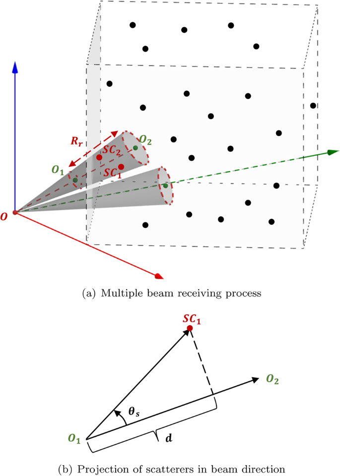

  

  Modeling of scanning process

• 2. Distance constraints locate each scatterer to its range bin. As shown in Fig. 3b, the distance is calculated by projecting the distance from each scatterer to the radar station onto the beam center axis. The distance constraint can be expressed as

  $$d = \left| {\overrightarrow {{O_{1} SC_{1} }} } \right|\cos \left( {\theta _{S} } \right) = \frac{{\overrightarrow {{O_{1} SC_{1} }} *\overrightarrow {{O_{1} O_{2} }} }}{{\left| {O_{1} O_{2} } \right|}}$$

  (4)
  $$|O_{1} (x,y,z)| < d < |O_{2} (x,y,z)|$$

  (5)

  where $\overrightarrow{O_1O_2}$ represents the vector of the range resolution in the direction of the beam center axis, $\overrightarrow{O_1SC_1}$ represents the vector from the starting point of the current range bin to the scatterer, d is the projection distance we calculated.

The above steps are repeated to realize the simulation of all the range bins in a single beam. It should be mentioned that for the transmitting beam, only the echo areas illuminated within the beam range need to be determined. The simulation of the whole volume scanning process is composed of beams with different elevation angles and azimuth angles.

3.3 Time series generation

In the actual radar detection, the echo pulse sequence that changes within a certain range bin is received. Due to the randomness of the size and location of the scatterers in the atmospheric field, the amplitude and phase are both random variables, so the sampling of the time series has great randomness. According to the theoretical research and observation, the power spectrum of most meteorological echoes with Gauss distribution [24, 25], so the time series I/Q signal is also a Gaussian distribution with zero mean value.

The coherent integration signal from of all scatterers in a single range bin is referred to as the composite signal. Each composite signal of the spectrum signal from all scatterers can be mathematically expressed as follows [9, 19]:

$$S\left( f \right) = \iiint {SC_{i} (f)d\theta d\varphi dr} + \aleph$$

(6)

where $SC_{i}$ represents the power spectrum signal of a single scatterer, echo signal of single range bin constructed by integrating all scatterer signals within range resolution, and $\aleph$ is the simulated thermal noise added.

Each SC in the 3D weather field represents the meteorological echo of each range bin detected by the actual radar, so we can recover its power spectrum signal by simulation. The spectrum signal of each SC can be expressed as

$$\begin{aligned} SC_{\text {i}}(f)=-ln(1-RND)\dfrac{P_i}{\sqrt{2\pi }\sigma _f}exp\left[ \dfrac{(f-f_d)^2}{2\sigma _f^2}\right] ,\ i=1,2,\ldots N \end{aligned}$$

(7)

where RND is a random variable that obeys uniform distribution between [0, 1], N is the number of scatterers, $\sigma _f$ refers to the spectral width, $\sigma _f=2W_i/\lambda$, $W_i$ is the velocity spectrum width, $f_d$ refers to Doppler frequency shift, $f_d=2V_i/\lambda$, $V_i$ is the average radial velocity. Frequency f related to PRF and pulse accumulation number expressed as

$$\begin{aligned}&f=-\dfrac{PRF}{2}+\dfrac{m\cdot PRF}{M},m=1,2,\ldots M \end{aligned}$$

(8)

where m is the sequence number of each pulse and M is the pulse accumulation number. In the PAWR simulator, the random phase is used to represent the phase information of the scatterer, and the phase spectrum $D_f=2\pi \cdot RND$.

$P_i$ is the average return power of each scatterer weighted by antenna gain, according to the Monte Carlo method [26], the sum of the contributions of each scatterer within a single range bin is used to determine the overall amount of backscattered energy. In the PAWR simulator, the echo intensity of a single range bin depends on the reflectivity factor of all scatterers in the range bin, the antenna gain and the coherent integration of the distance, and the weighting functions are used to calculate the total energy returned by each range bin without considering the system loss and radar peak power difference. The expression of the weighting functions are as follows:

$$\begin{aligned} P_i=\frac{{10}^{\left( \frac{Z_i}{10}\right) }G_t\left( \theta _t^i\right) G_r\left( \theta _r^i\right) }{\sum _{i=1}^{N}{G_t\left( \theta _t^i\right) G_r\left( \theta _r^i\right) }},i=1,2,\ldots N \end{aligned}$$

(9)

where $Z_i$ is the reflectivity factor of each scatterer in the range bin. $\theta _t^i$ and $\theta _r^i$ are the angles between each scatterer and the central axis of the transmitting beam and the central axis of the receiving beam in the vertical direction, respectively. $G_t$ and $G_r$ are the transmitting gain and receiving gain of each scatterer at this position, $G_t=G_{t0}\cdot cos\theta _t^i$ , and $G_r=G_{r0}\cdot cos\theta _r^i$ . The time series I/Q can be obtained after IDFT by combining the phase spectrum and the reconstructed power spectrum signal, which is expressed as

$$X_{M} = I_{M} + jQ_{M} = \sum\limits_{{i = 1}}^{M} {\left( {\sqrt {S_{f} } \cos D_{f} + \sqrt {S_{f} } \sin D_{f} } \right)} \cdot \exp \left( {\frac{{j2\pi mi}}{M}} \right)$$

(10)

were the time series $X_M$ is the simulated echo signal, and the spectral moment estimation uses the PPP method [27] to calculate the average radial velocity and spectral width from the signal. Repeat the above methods for each range bin to obtain the time series and spectral moments of all scanning areas.

3.4 Antenna characteristics

The linear array antenna pattern model is employed in this paper to describe the antenna pattern. The antenna pattern is expressed as [28]:

$$F(\theta ) = \cos ^{{\tfrac{{EF}}{2}}} (\theta ) \cdot \sum\limits_{{m = 1}}^{M} {I_{m} } e^{{j\tfrac{{2\pi }}{\lambda }x_{m} \left( {\sin (\theta ) - \sin \left( {\theta _{0} } \right)} \right)}}$$

(11)

where EF is the element factor. In this paper, all elements are set to have the same element factor, where M is the number of elements and $I_m$ is the complex voltage of each element; the complex voltage of all elements is the same, $I_m=1$. $\text {}\lambda \text {}$ is the radar wavelength and $x_m$ refers to as the position of the array element which is calculated as

$$\begin{aligned}x_m=[m-0.5(m+1)d],m=1,2,\ldots ,M \end{aligned}$$

(12)

where d is the element spacing, $d=\lambda /2$. To prevent the occurrence of grating lobes, the element spacing is generally not more than half of the wavelength in the design.

In the PAWR simulator, the antenna characteristics of linear phased array are reflected by the antenna pattern. To simplify, the switch between transmitting and receiving states in PAWR is realized by controlling the number of open and close array elements. It is easy to find that beamwidth and antenna gain change with scanning angle and transmitting and receiving states. The beam width is represented by the antenna pattern as

$$\begin{aligned}\varphi _V=\dfrac{k\lambda }{Lcos\theta _0} \end{aligned}$$

(13)

where $\varphi _V$ is considered as 3dB vertical beam width under uniform aperture irradiation, where k is the beam width factor, $k=0.886$, L is the antenna aperture length, $L=Md$. Similarly, for the phased array radar with uniform aperture and radiation efficiency of 1, the antenna gain can be expressed as [29]

$$G_{0} = 10\lg \frac{{32000}}{{\theta _{H} \varphi _{V} }}$$

(14)

where $\theta _{H}$ is the horizontal beam width, in 1D PAWR, $\theta _{H}$ does not change with scanning, which is set to a fixed value ($\theta _H=1^\circ$), $G_0$ is the antenna gain in the initial state ($\theta _0=0^\circ$) and then recalculated with the change of scanning angle during volume scanning.

Finally, we give the specific algorithm flow of the simulation model in Fig. 4.

Fig. 4

Algorithm flow chart of volume scanning simulation

4 Examples and discussion

In order to demonstrate the precision and adaptability od the PAWR simulator as well as the effects on data quality under various scanning strategies, this section present three examples. The three examples are based on a typical tornado weather scenario modeling.

4.1 Verification of PAWR simulator

We selected NEXRAD II level data from a tornado process monitored by the Kentucky (KHPX) WSR-88D radar at 3:33:22 on December 11, 2021, to generate a 3D weather field with a resolution of 0.1 km × 0.1 km × 0.5 km. We choose the scanning results of WSR-88D radar as a reference field to verify the effect and accuracy of the simulator. The PAWR related modules in the simulator are closed to avoid the simulation differences caused by the antenna of the phased array, and the general radar parameter configuration is retained. The scanning strategy adopts the VCP212 mode consistent with WSR-88D, which is used for some extreme weather such as strong convection. The system parameter configuration of general radar is shown in Table 1. Most of the parameters are obtained by reading NEXRAD II level data, and the antenna gain is calculated according to Formula (14). Figure 5 shows the simulation results of the PAWR simulator, and Fig. 5a, b is reflectivity PPIs for reference field and simulated volume scanning, respectively.

Table 1 General radar system parameters

Fig. 5

The PPI display of reflectivity factor in simulated field and reference field at 0.44° elevation cut

It can be found from the PPI that the display of the simulation field is somewhat “fuzzy” compared with the reference field display, this phenomenon is mainly to obtain the resolution of the original data that does not meet our needs, and the interpolation algorithm smoothies the NEXRAD II data. But the simulation field keeps a high consistency with the reference field in the overall structure of the echo, especially at the triangular marker, it can be found that the simulation field retains the same tornado feature as the reference field, namely the typical hook echo. Figure 6 shows the distribution of complete areas’ reflectivity of the simulation field and reference field. Overall, the simulation and reference fields maintain a consistent trend, especially in areas larger than 20dBZ. The simulation field below 20dBZ is lower than the reference field as a whole, on the one hand, because the “cone of silence” appears in the center of the simulation field, as can be seen from Fig. 5, on the other hand, the loss of the simulation process (data smoothing) makes the effective data of the simulation field less than the reference field (less than 20dBZ areas).

Fig. 6

The distribution of complete areas reflectivity of the simulation and reference fields

4.2 PAWR volume scan

4.2.1 Single elevation cut example

In this section, the parameters of the phased array in the PAWR simulator are reconsidered, and the single elevation cut of S-band 1D PAWR is simulated. The parameter configuration of the phased array weather radar is shown in Table 2, and the scanning strategy configuration is shown in Table 1.

Table 2 System parameters of the simulated 30-elements PAWR

Here, we choose the lowest elevation cut for scanning simulation. Figure 7 shows the spectral moments of the simulation field and the reference field, where the reference field for the elevation cut (0.44°), and the simulation field for the elevation cut (0.44°). In Fig. 7b, c, the triangular marker represent a single range bin. After spectrum reconstruction, Fig. 7d shows the time series and Doppler spectrum at the triangular marker, and the corresponding information of all scatterers in a single range bin is given in Table 3, the average radial velocity of simulation is $V_{sim}=-28.9$ m/s, and the spectrum width of simulation is $W_{sim}=2.9$ m/s.

Fig. 7

The simulation field and spectral moments at the lowest elevation cut, and comparison with the reference field

Table 3 Scatterers’ spectral moments within a single range bin in a volume scan simulation

4.2.2 Volume scan

Further simulation of the complete volume scanning process, the purpose of this part of the simulation is to compare and analyze the phased array data and the reference field, and to verify its consistency with the actual PAWR observation experiment results. Figure 8 shows the PPI display of the volume scanning process for the reference field and simulation field. And Table 4 shows the running time of the volume scanning process.

Fig. 8

From top to bottom are the PPI display of the simulation field volume coverage pattern at the elevation cuts (0°, 3°, 6°, 9°), and comparison with reference field at the elevation cuts (0.44°, 1.23°, 3.07°, 5.07°)

Table 4 The running time of simulation

Without considering the effects of range ambiguity and velocity ambiguity in the PAWR simulator, a higher PRF is set. In this paper, the detection range of simulated PAWR is far less than that of WSR-88D radar. To make PAWR scan to the same echoes areas as WSR-88D radar, we scaled down the spatial scale of the weather echo in the process of drawing PPI. We can find that the echo position of the simulation field and the reference field in the PPI display is not completely consistent, because the relative position between the simulated radar and the weather echo cannot be guaranteed to be consistent with the actual radar when the weather echo is scaled in equal proportion, which has does not affect the analysis of the echo structure and intensity change. It can be seen that the simulated spectral moments, including reflectivity, average radial velocity and spectral width, are close to the reference field in the overall structure and intensity. At the same time, we can also find that the echo areas scanned by PAWR are higher than that of the reference field, especially with the elevation of the scanning elevation angle, this situation is more obvious. This is because the 3° beam width used by PAWR here will receive more echo information than the 1° beam width of WSR-88D. Secondly, the beam broadening effect of the PAWR will increase with the increase in the scanning angle, which will be discussed emphatically in the next section.

We compare the scanning results of PAWR and WSR-88D radars using the reflectivity of the lowest elevation cuts. When compared to other elevation cuts, the echo areas scanned by the two radars at the lowest elevation cuts are the closest. The probability density distribution of reflectivity is depicted in Fig. 9.

Fig. 9

Probability density distribution of reflectivity of two radars at the lowest elevation cut

There are obvious differences between PAWR and WSR-88D radar in the echo near 20 dBZ and the echo below 0 dBZ. According to the observation experiment, the echo intensity is divided into three kinds of intensity: weak echoes (< 30 dBZ), medium echoes (10−30 dBZ), and strong echoes (> 30 dBZ). For further data analysis, Table 5 shows the proportion of different intensity echoes of the two radars (the calculation is based on the proportion of current grade echoes in their effective echoes); PAWR has a lower proportion in strong echo than WSR-88D radar, a higher proportion in medium echo and a lower proportion in weak echo, which is close to the results of field observation experiments [30]. From the perspective of the antenna, it is due to the smoothing effect of the PAWR wide beam and the low antenna gain. On the one hand, the strong echo areas and the weak echo areas are smoothed in the detection process, which increases the areas of medium echo. On the other hand, the antenna gain of PAWR is lower than that of the WSR-88D parabolic reflector system, which reduces the sensitivity of PAWR and the detection ability of PAWR for weak echo [31].

Table 5 The proportion of different intensity echoes of two radars

4.3 Different PAWR

In this section, the PAWR simulator of S-band PAWR system with different array elements and different array angles v is represented. The purpose of this part of the simulation is to study the influence of the number of elements and the angle of the array on the simulation scanning results.

We simulated two kinds of PAWR: 30-elements and 60-elements. The radar parameters are configured in Tables 2 and 6. Two kinds of PAWR scan the same echo areas with different array angles v. In fact, the change of array angle can be regarded as the change of scanning angle. Figure 10 shows the reflectivity generated by simulation of two kinds of PAWR at different array angles and their corresponding antenna pattern, the array angles are set to 5° and 45°, respectively.

Table 6 System parameters of the simulated 60-elements PAWR

Fig. 10

The PPI display of reflectivity and corresponding antenna pattern for 30-elements and 60-elements PAWR at different array angles

The simulated radar reflectivity shows that the 30-elements PAWR has a more noticeable smoothing effect than the 60-elements PAWR in the hook echo near the triangle areas, and this part of the detail has been completely lost. Figure 11 shows the probability density distribution of reflectivity data in Fig. 10 after statistical analysis; we can further see that the scanning results of 30-elements at 45° array angle and 5° array angle have obvious changes, while the scanning results of 60-elements at 45° array angle and 5° array angle have no obvious changes. Similarly, Table 7 summarizes the error statistics of reflectivity data of different linear arrays in this simulation; the reference field in Fig. 7 is used as the calculation standard. From the results, it can be seen that in terms of data quality, 60 array elements will be better. In general, the 30-elements has a wider beam width than the 60-elements, which is unfavorable for the fine observation of the structure of weather scenes such as tornadoes. At the same time, a wider beam width will bring a more serious beam broadening effect, which will be difficult for us to analyze data in the later stage.

Fig. 11

Probability density distribution of reflectivity of two kinds of PAWR at different array angles

Table 7 Summary of error statistics under simulation

5 Conclusions

The scanning model and the SPARC framework, which were both developed by Schvartzman et al. [13], are combined in this phased array weather radar (PAWR) simulator, which moves the simulation process from two-dimensional to three-dimensional data input. The Lagrange SC framework, which Cheong et at. [11] demonstrated, is combined with the beam pattern to introduce the phased array antenna pattern, which reflects the beam pattern characteristics of the phased array. We demonstrate the application of this method for spectrum reconstruction using the time series generating method provided by Zrnic [9]. The spectral moment parameter velocity and spectral width are examples that are obtained via the PPP approach.

To eliminate the effects of the phased array beam characteristics input to the data, simulations construct a 3D filed using NEXRAD II data rather than phased array radar observation data. Additionally, since NEXRAD II data are used directly as input to weather processes, this method allows us to complete the scanning simulation of all without incurring the additional time and computational costs of using sophisticated methods like a numerical prediction model and only simulating a volume with a single resolution. The radar system parameters are added to the scanning model and time series modeling. To establish the relationship between the simulated scanning weather echoes and the radar system parameters, the radar system parameters are added to the scanning model and time series modeling. In the same weather scenario, we evaluated the simulation performance of the PAWR simulator and provided two examples. The findings demonstrate that this approach is not only appropriate for phased array radar but also exhibits well congruence with the real WSR-88D radar after closing the phased array characteristic module. Next, we simulated the complete PAWR volume scanning and compared it with the results of WSR-88D radar scanning. The comparison results show that the simulator is capable of simulating a phased array radar’s whole scanning process and producing the relevant spectral moments. It has also been established that the phased array’s wide beam will have a noticeable smoothing effect in the scanned echo areas. At the same time, a wide beam’s reduction in beam gain will make it harder to detect weak echoes, and the receiving echo regions will grow as a result of the phased array’s wide beam. Compared to WSR-88D radar, this was particularly pronounced at high elevation angle. Additionally, the two different types of PAWR scan the identical echo areas at various elements and array angles were contrasted in the samples. The results show that the 60-elements PAWR retains more echoes structure than 30-elements, and the influence of the beam broadening effect on high scanning angle will also be significantly reduced. At the same time, the scanning angle is correlated with the array angle. When scanning at a high elevation cut, the array angle is changed to reduce the scanning angle and reduce the influence of the beam broadening effect.

Currently, the PAWR simulator focuses on the 1D PAWR, which is most widely used in meteorological service. The PAWR simulator system structure will be improved in the following work in order to model the two-dimensional phased array scanning process. Additionally, the impact of phased array characteristics on the measurement of the polarization parameter during scanning is then further investigated by combining the polarization parameter simulation approach with the PAWR simulator.

References

B. Isom, R. Palmer, R. Kelley, J. Meier, D. Bodine, M. Yeary, B.-L. Cheong, Y. Zhang, T.-Y. Yu, M.I. Biggerstaff, The atmospheric imaging radar: simultaneous volumetric observations using a phased array weather radar. J. Atmos. Ocean. Technol. 30(4), 655–675 (2013). https://doi.org/10.1175/JTECH-D-12-00063.1
J.M. Kurdzo, F. Nai, D.J. Bodine, T.A. Bonin, B. Isom, R.D. Palmer, B.L. Cheong, J. Lujan, A. Mahre, A.D. Byrd, Observations of severe local storms and tornadoes with the atmospheric imaging radar. Bull. Am. Meteorol. Soc. 98(5), 915–935 (2017). https://doi.org/10.1175/BAMS-D-15-00266.1
M.M. French, H.B. Bluestein, I. PopStefanija, C.A. Baldi, R.T. Bluth, Mobile, phased-array, doppler radar observations of tornadoes at x band. Mon. Wea. Rev. 142(3), 1010–1036 (2014). https://doi.org/10.1175/MWR-D-13-00101.1
P.L. Heinselman, D.L. Priegnitz, K.L. Manross, T.M. Smith, R.W. Adams, Rapid sampling of severe storms by the national weather radar testbed phased array radar. Weather. Forecast. 23(5), 808–824 (2008). https://doi.org/10.1175/2008WAF2007071.1
E.N. Anagnostou, W.F. Krajewski, Simulation of radar reflectivity fields: algorithm formulation and evaluation. Water Resour. Res. 33(6), 1419–1428 (1997). https://doi.org/10.1029/97WR00233
G. Haase, S. Crewell, Simulation of radar reflectivities using a mesoscale weather forecast model. Water Resour. Res. 36(8), 2221–2231 (2000). https://doi.org/10.1029/2000WR900041
W.F. Krajewski, R. Raghavan, V. Chandrasekar, Physically based simulation of radar rainfall data using a space-time rainfall model. J. Appl. Meteorol. 32(2), 268–283 (1993). https://doi.org/10.1175/1520-0450(1993)032<0268:PBSORR>2.0.CO;2
C. Augros, O. Caumont, V. Ducrocq, P. Tabary, Development and validation of a full polarimetric radar simulator. In: 36th Conference on Radar Meteorology, Breckenridge, vol. 387 (2013)
D.S. Zrnić, Simulation of weatherlike doppler spectra and signals. J. Appl. Meteorol. 14(4), 619–620 (1975). https://doi.org/10.1175/1520-0450(1975)014<0619:SOWDSA>2.0.CO;2
G. Galati, G. Pavan, Computer simulation of weather radar signals. Simul. Pract. Theory 3(1), 17–44 (1995). https://doi.org/10.1016/0928-4869(95)00009-I
B.L. Cheong, R.D. Palmer, M. Xue, A time series weather radar simulator based on high-resolution atmospheric models. J. Atmos. Ocean. Technol. 25(2), 230–243 (2008). https://doi.org/10.1175/2007JTECHA923.1
A.D. Byrd, I.R. Ivić, R.D. Palmer, B.M. Isom, B.L. Cheong, A.D. Schenkman, M. Xue, A weather radar simulator for the evaluation of polarimetric phased array performance. IEEE Trans. Geosci. Remote Sens. 54(7), 4178–4189 (2016). https://doi.org/10.1109/TGRS.2016.2538179
D. Schvartzman, C.D. Curtis, Signal processing and radar characteristics (sparc) simulator: a flexible dual-polarization weather-radar signal simulation framework based on preexisting radar-variable data. IEEE J. Sel. Top. Appl. Earth Observ. 12(1), 135–150 (2019). https://doi.org/10.1109/JSTARS.2018.2885614
S.M. Torres, D. Schvartzman, A simulation framework to support the design and evaluation of adaptive scanning for phased-array weather radars. J. Atmos. Ocean. Technol. 37(12), 2321–2339 (2020). https://doi.org/10.1175/JTECH-D-20-0087.1
C. Capsoni, M. D’Amico, A physically based radar simulator. J. Atmos. Ocean. Technol. 15(2), 593–598 (1998). https://doi.org/10.1175/1520-0426(1998)015<0593:APBRS>2.0.CO;2
C. Capsoni, M. D’Amico, R. Nebuloni, A multiparameter polarimetric radar simulator. J. Atmos. Ocean. Technol. 18(11), 1799–1809 (2001). https://doi.org/10.1175/1520-0426(2001)018<1799:AMPRS>2.0.CO;2
V. Chandrasekar, V.N. Bringi, Simulation of radar reflectivity and surface measurements of rainfall. J. Atmos. Ocean. Technol. 4(3), 464–478 (1987). https://doi.org/10.1175/1520-0426(1987)004<0464:SORRAS>2.0.CO;2
F. Nai, J. Boettcher, C. Curtis, D. Schvartzman, S. Torres, The impact of elevation sidelobe contamination on radar data quality for operational interpretation. J. Appl. Meteorol. Climatol. 59(4), 707–724 (2020). https://doi.org/10.1175/JAMC-D-19-0092.1
A. Lupidi, C. Moscardini, F. Berizzi, M. Martorella, Simulation of x-band polarimetric weather radar returns based on the weather research and forecast model. In: 2011 IEEE RadarCon (RADAR), pp. 734–739 (2011). https://doi.org/10.1109/RADAR.2011.5960635
R.A. Fulton, Wsr-88d polar-to-hrap mapping. Hydrologic Research Laboratory, Office of Hydrology, National Weather Service Tech. Memo 34 (1998)
C.G. Mohr, R.L. Vaughan, An economical procedure for cartesian interpolation and display of reflectivity factor data in three-dimensional space. J. Appl. Meteorol. Climatol. 18(5), 661–670 (1979). https://doi.org/10.1175/1520-0450(1979)018<0661:AEPFCI>2.0.CO;2
J. Zhang, K. Howard, J.J. Gourley, Constructing three-dimensional multiple-radar reflectivity mosaics: examples of convective storms and stratiform rain echoes. J. Atmos. Ocean. Technol. 22(1), 30–42 (2005). https://doi.org/10.1175/JTECH-1689.1
R.J. Doviak et al., Doppler Radar and Weather Observations (Courier Corporation, Chelmsford, 2006)
L.H. Janssen, G.A. Van Der Spek, The shape of doppler spectra from precipitation. IEEE Trans. Aerosp. Electron. Syst. AES 21(2), 208–219 (1985). https://doi.org/10.1109/TAES.1985.310618
S. Dai, X. Li, Z. Bu, Y. Chen, J. He, M. Li, M. Xiong, Signal simulation of dual-polarization weather radar and its application in range ambiguity mitigation. Atmosphere 13(3), 432 (2022). https://doi.org/10.3390/atmos13030432
N. Metropolis, S. Ulam, The Monte Carlo method. J. Am. Stat. Assoc. 44(247), 335–341 (1949). https://doi.org/10.1080/01621459.1949.10483310. (PMID: 18139350)
D.S. Zrnic, Estimation of spectral moments for weather echoes. IEEE Trans. Geosci. Electron. 17(4), 113–128 (1979). https://doi.org/10.1109/TGE.1979.294638
A.D. Brown, Electronically Scanned Arrays MATLAB® Modeling and simulation (CRC Press, Boca Raton, 2017)
M.I. Skolnik, Radar Handbook (McGraw-Hill Education, New York, 2008)
C. Wu, L. Liu, Z. Zhang, Quantitative comparison algorithm between the s-band phased array radar and the Cinrad/Sa and its preliminary application. Acta Meteorol. Sin. 72, 390–401 (2014)
D.J. Bodine, J.M. Kurdzo, C.B. Griffin, R.D. Palmer, B. Isom, F. Nai, A. Mahre, M. Yeary, T.-Y. Yu,D Overview of a decade of field experiments with the atmospheric imaging radar. In: 2022 IEEE Radar Conference (RadarConf22), pp. 1–6 (2022). https://doi.org/10.1109/RadarConf2248738.2022.9764270
Acknowledgements
The authors would like to express their sincere thanks to the editors and anonymous reviewers.
Funding
This work was supported by Natural Science Foundation of China (41575022) and the Natural Science Foundation of Si Chuan(2022NSFSC0214 and 2022NSFSC0209).
Author information
Authors and Affiliations
Contributions
X.L. and Z.L. designed the algorithm; Z.L. and S.D. performed programming to obtain algorithm results; X.L., F.L. and S.T. analyzed the results; Z.B., J.H. and S.Z. supervised the work and provided comments on the results; Z.L. wrote this paper; X.L. and C.W. revised the paper. All authors have read and agreed to the published version of the manuscript.
Corresponding author
Ethics declarations
Ethics approval and consent to participate
Not applicable.
Consent for publication
Competing interests
The authors declare that they have no competing interests.
Additional information
Publisher's Note
Springer Nature remains neutral with regard to jurisdictional claims in published maps and institutional affiliations.
Rights and permissions
Open Access This article is licensed under a Creative Commons Attribution 4.0 International License, which permits use, sharing, adaptation, distribution and reproduction in any medium or format, as long as you give appropriate credit to the original author(s) and the source, provide a link to the Creative Commons licence, and indicate if changes were made. The images or other third party material in this article are included in the article's Creative Commons licence, unless indicated otherwise in a credit line to the material. If material is not included in the article's Creative Commons licence and your intended use is not permitted by statutory regulation or exceeds the permitted use, you will need to obtain permission directly from the copyright holder. To view a copy of this licence, visit http://creativecommons.org/licenses/by/4.0/.
About this article
Cite this article
Li, X., Lin, Z., Bu, Z. et al. Volume scan modeling simulator of a 1D phased array weather radar. EURASIP J. Adv. Signal Process. 2023, 79 (2023). https://doi.org/10.1186/s13634-023-01039-6
Received:
Accepted:
Published:
DOI: https://doi.org/10.1186/s13634-023-01039-6