- Research Article
- Open access
- Published:
Low-Complexity Design of Frequency-Hopping Codes for MIMO Radar for Arbitrary Doppler
EURASIP Journal on Advances in Signal Processing volume 2010, Article number: 319065 (2010)
Abstract
There has been a recent interest in the application of Multiple-Input Multiple-Output (MIMO) communication concepts to radars. Recent literature discusses optimization of orthogonal frequency-hopping waveforms for MIMO radars, based on a newly formulated MIMO ambiguity function. Existing literature however makes the assumption of small target Doppler. We first extend the scope of this ambiguity function to large values of target Doppler. We introduce the concept of hit-matrix in the MIMO context, which is based on the hit-array, which has been used extensively in the context of frequency-hopping waveforms for phased-array radars. We then propose new methods to obtain near optimal waveforms in both the large and small Doppler scenarios. Under the large Doppler scenario, we propose the use of a cost function based on the hit-matrix which offers a significantly lower computational complexity as compared to an ambiguity based cost function, with no loss in code performance. In the small Doppler scenario, we present an algorithm for directly designing the waveform from certain properties of the ambiguity function in conjunction with the hit-matrix. Finally, we introduce "weighted optimization" wherein we mask the cost function used in the heuristic search algorithm to reflect the properties of the required ambiguity function.
1. Introduction
MIMO radar is a recent evolution of radar that utilizes multiple transmitters and receivers [1, 2]. MIMO radar waveforms can have any degree of coherence with each other, ranging from complete coherence (in which case it is equivalent to a phased-array radar) to complete incoherence (orthogonality). The choice of radar waveforms [3] plays an important role in the resolution characteristics of the radar. The optimization of radar waveforms for the phased-array radar, which is also viewed as single-input multiple-output (SIMO) radar, focuses on obtaining a desirable ambiguity function in terms of range and Doppler resolutions. On the other hand, MIMO radars provide spatial resolution and spatial diversity in addition to range and Doppler resolution.
Frequency-hopping codes have been used in pulse compression radars [4] because of their highly desirable ambiguity properties. The design of frequency-hopping codes for SIMO radars to obtain desired ambiguity functions [5] has been well studied. A method to design discrete frequency-coding waveforms for the netted radar has been proposed in [6] and a modified Genetic algorithm to design orthogonal discrete frequency-coding waveforms for MIMO radar has been presented in [7]. The hit-array [8, 9] has also been extensively used for waveform design in the SIMO context.
Recently, Chen and Vaidyanathan [10, 11] have dealt with the design of frequency-hopping codes for MIMO case based on the optimization of a newly formulated MIMO ambiguity function [12]. Their approach to designing radar waveforms is to first parameterize these waveforms and then apply simulated annealing to find a near-optimal set of parameters using a "cost function" that allows comparison of different parameter sets. The formulation assumes small target Doppler resulting in a simpler cost function. This formulation, however, is inapplicable in the presence of large target Doppler.
In this paper, we first extend the scope of this ambiguity function to large values of target Doppler, and then introduce the concept of hit-matrix in the MIMO context. Next, we propose new methods to obtain optimal waveforms in both the large Doppler and small Doppler scenarios. In the case of large Doppler, we propose a cost function based on the hit-matrix which offers a significantly lower computational complexity as compared to an ambiguity-based cost function, with no loss in code performance. In the small Doppler case, we present an algorithm for directly designing the waveform from certain properties which can be obtained from the ambiguity function in conjunction with the hit-matrix. Finally, we introduce a "weighted optimization" wherein we weight the cost function, used in the heuristic search algorithm, to reflect the properties of the required ambiguity function.
In Section 2, we present our model for MIMO radar and frequency-hopping waveforms. In Section 3, we reformulate Chen and Vaidyanathan's MIMO ambiguity function such that it is applicable to any general value of Doppler. In Section 4, we describe the use of hit-matrix as an optimization tool. The hit-matrix corresponds to a digitized version of the ambiguity function which is relatively simple to compute. In Section 5, using a hit-matrix-based cost function, we use simulated annealing to search for the best frequency-hopping codes under the large Doppler scenario. In Section 6, we present an algorithm for directly obtaining a waveform corresponding to a good ambiguity function in the small Doppler case. In Section 7, we propose a method to obtain waveforms satisfying certain conditions on the ambiguity function. A heuristic search performed using a weighted cost function, with the weights representing conditions on ambiguity function, illustrates our proposed method. Section 8 concludes this paper.
2. System Model
2.1. MIMO Radar Model
Consider a monostatic MIMO radar that contains  transmitters and
  receivers with their antennas configured as uniform linear arrays, as shown in Figure 1. We assume a point target and also that the target, transmitters and receivers lie in the same 2D plane. Let
  and
and  represent the spacing between consecutive transmitters and receivers, respectively, and let
  . We define the spatial frequency of the target as

where  is the target angle with respect to the broadside direction and
  is the wavelength of the RF carrier of the transmitted waveforms. Let
  and
and  be the target delay (which is a measure of target range) and Doppler frequency (a measure of target velocity), respectively. The spatial frequency
  corresponds to the angular location of the target with respect to the arrays of the radar. Let
  ,
,  represent the
  transmitter waveforms. Then, the waveform received at the
  th receiver antenna can be expressed as [11]


Transmitters and receivers in a MIMO radar (MF = Matched filter).
2.2. Frequency-Hopping Waveforms
Frequency-hopping signals are good candidates for the radar waveforms because they are easily generated and have constant modulus. The waveforms can be represented as (see Figure 2)

where

Here,  is the
  th element of the matrix
  and it can assume values from the set
  , where
  is the total number of frequency hops available. As shown in Figure 2, each transmitter waveform
  consists of a stream of
  identical pulses
  . Each pulse in turn contains
  constant amplitude frequency subpulses each having width
  and frequency
  . Here we only concern ourselves with waveforms that are orthogonal at zero Doppler and zero delay mismatch, that is,


The structure of frequency-hopping waveforms.
To attain orthogonality, we impose the following conditions on the waveforms [11]:

Orthogonal waveforms result in a uniform gain in all directions, which is a key aspect of detection using MIMO radars. For fixed  and
and  , these waveforms can be completely described by the code matrix:

and the pulse spacing vector:

The pulse spacing vector plays a role in shaping the Doppler resolution of the waveforms. In this paper, however, we will not be dealing with optimization of this vector.
3. MIMO Radar Ambiguity Function
The resolution of a radar system is determined by the response to a point target in the matched filter output. This response can be characterized by a function called the ambiguity function. The traditional Woodward ambiguity function for a SIMO radar is given as

In the above expression,  and
and  represent the delay and Doppler mismatch at the receiver, respectively. The ideal ambiguity function should be sharp around the region of zero-mismatch, that is,
  . This idea has been extended to the MIMO case in [11]. Consider the expression for the received signal in a MIMO radar given in (2). Let
  represent the true parameters of a target, and let
  be the assumed parameters at the receiver. The summed match filter output is given as

In the above expression, the second term corresponds to the ambiguity function when only one receiver is present, while the first term brings out the effect of having multiple receivers. To simplify the ambiguity function and the waveform design problem, the first term can be decoupled from the above expression. The resulting expression is termed the "MIMO ambiguity function". We can now consider ( ) to be the delay mismatch and (
 ) to be the Doppler mismatch, and rewrite the expression. The MIMO radar ambiguity function is thus given as [11]

where  and
and  represent the Doppler and delay mismatch at the receiver,
  represents the target's true spatial frequency,
  represents the assumed spatial frequency at the receiver, and
  represents the cross-ambiguity function between the waveforms
  and
and  , given by

For frequency-hopping waveforms (see Figure 2), (12) becomes

where

We assume that the maximum expected target delay is less than the time interval between any two consecutive pulses of each transmitter waveform as they are colocated. This assumption implies that  due to which

and hence

 is the cross-ambiguity between two individual pulses of different waveforms (
 and
and  ) and can be expanded as

where

represents the ambiguity function of the rectangular pulse  . In [11], the Doppler is assumed to be small (
 ) due to which (17) reduces to

In the subsequent sections, we do not assume small Doppler and work with (17). We next describe the hit-matrix formalism in Section 4 and waveform optimization for the large Doppler case in Section 5.
4. The Hit-Matrix Formalism
The hit-array has been introduced as a tool to analyze frequency-hopping waveforms in [9]. The central concept in this formulation is that of a "hit", which occurs when the received pattern has been shifted in the time-frequency space in such a way that it overlaps with the original pattern at exactly one time-frequency position. In this section, we extend the hit-array to the hit-matrix, which is applicable to frequency-hopping codes for MIMO radar under the large Doppler scenario. We define the hit-matrix for the code matrix  as
as


where

and  refers to the Kronecker delta function. The concept of hit-array was used in phased array as well as multiple access radars for approximating auto- and cross-ambiguity functions. The hit-array is either auto-hit-array (
 ) or cross-hit-array (
 ) as defined below (see (24)). The hit-matrix
  can be obtained by summing the individual auto- and cross-hit arrays as follows:

where

As an example, consider the code matrix:

Here  ,
,  , and
, and  . The cross-hit arrays for this code are

and the resulting hit-matrix is

Ambiguity Function and the Hit-Matrix
We now describe how the hit-matrix of a frequency-hopping code relates to its ambiguity function. Consider the MIMO radar ambiguity function in (11) which, in view of (16) and (17), can be expressed as

where

represents the ambiguity between two pulses and

is the cross-ambiguity between the  th subpulse of
  and the
  th subpulse of
  . A plot of
  is shown in Figure 3. The position of its peak is
  . Along the
  -axis, this function drops to zero at a shift of
  from
from  , and along the
  -axis, it falls by roughly 6 dB relative to the peak at a shift of
  from
from  . Hence most of the energy of each subpulse ambiguity function is located within an area of
  around
  . For different values of
  , the shape of
  remains the same, and only the position of its peak in the delay-Doppler space changes. The set of possible values of
  is given as

The number of 4-tuples  for which
  peaks at the position
  is
is

Thus each element of the hit-matrix corresponds to the number of functions  centered at the same point in the delay-Doppler space. The
  different functions
  for different values of the 4-tuple
  are the building blocks of the overall MIMO ambiguity function, and the distribution of the positions of their peaks in the delay-Doppler space plays a key role in determining the shape of the overall ambiguity function. The value of
  corresponds to the height of the mainlobe in the ambiguity function and is constant for a given code matrix size. The values of
  outside of
  correspond to sidelobes in the ambiguity function centered at
  . The higher these values of
  , the higher will be the corresponding sidelobes. Also, since the spatial frequency parameters
  and
and  appear as complex exponential weights in the summation of (29), a reduction in the values of the hit-matrix outside of
  will result in a corresponding reduction in sidelobes along the spatial frequency dimensions as well.

Cross-ambiguity between subpulses,  .
.
5. Waveform Design for Large Doppler
We now describe how frequency-hopping codes can be optimized under the large Doppler scenario to yield a desired ambiguity function. Since the second product term in the right-hand-side of (28) is not dependent on the choice of code matrix  , we only concern ourselves with the optimization of the first term
  . To apply heuristic search algorithms like simulated annealing, we require a cost function that allows the desirability of different codes to be compared. Following the formulation of [11], a cost function for the large Doppler case is given as follows:

It can be shown that the height of the peak in  at
at  is constant, and hence this cost function favors codes that have their sidelobes flattened out over the delay, Doppler and spatial frequency dimensions. Increasing the value of
  increases the penalty on higher sidelobes.
  can be evaluated for each code using Riemann sums with a sufficient number of bins instead of integrations. However, this results in a high computational complexity which increases as
  , where
  is the time-bandwidth product of the code.
Now, consider the elements of the hit-matrix  . From (22),
  , and as explained in the previous section, it corresponds to the height of the mainlobe in the ambiguity function, and
  outside of
  correspond to sidelobes in the ambiguity function. The higher these values of
  , the higher will be the corresponding sidelobes. This motivates us to choose the following cost function based on the hit-matrix:

which favors the codes that have their sidelobes flattened out over the delay, Doppler and spatial frequency dimensions. Evaluation of  is far less computationally intensive than
  , and increases only as
  . This allows the heuristic search algorithms using this cost function to rapidly traverse the code space, thereby allowing good codes to be found faster.
We now describe how we apply simulated annealing using  . We use a slightly modified form of simulated annealing called quantum-simulated annealing, which allows faster convergence. The quantum-simulated annealing parameters are temperature (
 ), rate of decrease of temperature (α), jump size (
 ) and rate of decrease of jump size (β). The algorithm is initialized with a value of
  and
and  , choosing α and β from
  . The steps of the algorithm are as follows.
-
(1)
Randomly draw a code matrix
 from
from  such that the code is orthogonal, that is,
  for
for  .
. -
(2)
Randomly draw
 from
from  .
. -
(3)
Set
 , and repeat steps 3(a) to 3(c)
  times.
-
(a)
Randomly draw
 from
from  and
and  from
from  .
. -
(b)
Select
 from
from  with
with  .
. -
(c)
Set
 . (At this point, we will have the original code
  , and
, and  obtained from the above steps.)
-
(a)
-
(4)
Randomly draw
 from
from  .
. -
(5)
If
 , then set
  .
. -
(6)
Set
 and
and  .
. -
(7)
If a sufficiently small value of
 has been obtained, terminate the algorithm. Otherwise, return to step 2.
 from
from  such that the code is orthogonal, that is,
  for
for  .
. from
from  .
. , and repeat steps 3(a) to 3(c)
  times.
 from
from  and
and  from
from  .
. from
from  with
with  .
. . (At this point, we will have the original code
  , and
, and  obtained from the above steps.)
 from
from  .
. , then set
  .
. and
and  .
. has been obtained, terminate the algorithm. Otherwise, return to step 2.
Consider as an example the optimization of frequency-hopping codes for  . The total number of possible codes of this size is
  . We found the number of Riemann sum bins, required for reasonable accuracy in the evaluation of
  for this code size, to be 100 each along the delay and Doppler dimensions, and 20 each along the two spatial frequency dimensions. Hence, while
  requires the computation and summation of
  terms per iteration,
  only needs 576 computations per iteration, resulting in a significant decrease in complexity.
5.1. Simulation Results
We present a number of examples to demonstrate the effectiveness of the hit-matrix-based cost function in designing good frequency-hopping codes. We have generated codes of various sizes by simulated annealing using both  and
and  at
at  . The code parameters used were
  ,
,  and
and  for each value of
  . Other parameters used were
  ,
,  and
and  . For simulated annealing, we set the parameters
  ,
,  ,
,  and
and  .
.
First, we consider the code obtained for  using
using  . The decrease in the cost with respect to the iterations of simulated annealing is shown in Figure 4. The final code obtained is

A plot of the hit-matrix of this code is shown in Figure 5 and a plot of  at
at  is shown in Figure 6. We observe that the ambiguity function of the above code has a very sharp mainlobe along the delay and Doppler dimensions, with 98% of the sidelobes lying 10 dB below the peak. Also note the visual similarity between the plots of hit-matrix and ambiguity function. Although it may appear that optimization using
  involves just the time and Doppler dimensions, it takes the spatial frequency into consideration as well. To show this, we consider values of
  at different values of
  .
.
-
(1)
 . The
. The  function can be expressed from (29) and (30) as follows:
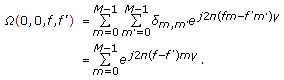 (36)
(36)The above expression is independent of the code matrix, and thus the ambiguity function in this form cannot be optimized along the spatial frequency dimensions at
 .
. -
(2)
 . Noting that each peak, given by
  , corresponds to a hit which is reflected in (34), and the ambiguity function consists of a weighted sum of hits with the weights being of the form
  , optimizing the hit-matrix is analogous to optimizing the upper bound on the ambiguity function along the spatial frequency dimensions.
 . The
. The  function can be expressed from (29) and (30) as follows:
 .
. . Noting that each peak, given by
  , corresponds to a hit which is reflected in (34), and the ambiguity function consists of a weighted sum of hits with the weights being of the form
  , optimizing the hit-matrix is analogous to optimizing the upper bound on the ambiguity function along the spatial frequency dimensions.
Decrease in  versus iterations of simulated annealing.

Plot of the hit-matrix of a code obtained from simulated annealing using  .
.

 for the code whose hit-matrix is shown in Figure 5.
We may point out here that the ambiguity function has a very low magnitude when  for all mismatched values of
  and
and  . To show this, various cuts of
  are shown in Figure 7 (at
  ). We now compare various codes obtained using
  and
and  . We take samples from the function
  and plot their empirical cumulative distribution function (ECDF), which show the percentage of samples of
  less than specified magnitudes. The highest peak has been normalized to 0 dB. Figure 8 shows the ECDF curves for various codes obtained at
  . Note that use of either cost function yields codes with similar ECDF curves. In Figure 9, we have plotted the magnitude of 95th percentile of
  for different codes, as a function of the time bandwidth products
  . Note that up to
  ,
,  and
and  both yield codes with a similar number of undesirable peaks. The curve corresponding to
  could not be extended beyond
  because of increasing computational complexity. However, using
  , codes with
  as high as 1200 (and higher) could be easily generated.

Various cuts of  for the code whose hit-matrix is shown in Figure 5.

Empirical CDF of  .
.

Magnitude of 95th percentile of  .
.
A large Doppler scenario will arise when a MIMO radar operating in the  band (27 GHz to 40 GHz) is expected to detect 5000 km class missile targets. To see how the cost function in [11], which assumes low Doppler, performs in comparison to the large Doppler cost function in (33), when Doppler frequency is a significant percentage of the signal bandwidth, we conducted the following simulation. We obtained the codes from the minimization of the two cost functions at
  , choosing the Doppler frequency as 25% of the transmitter waveform bandwidth for three different values of
  . Figure 10 gives the ECDF curves of the corresponding
  . Note from the plots that the large Doppler cost function yields an improvement of 0.5 dB for
  and 1.0 dB for
  at 90%. We may point out here that the bandwidth increases with increasing
  , and accordingly the Doppler frequency goes up as it is 25% of the bandwidth.

Empirical CDF of  for the codes obtained with two different cost functions.
6. Waveform Optimization for Small Doppler Case ( )
)
 )
)As derived in [11], for the small Doppler condition ( ) and under the assumption of no range folding, we have from (16) and(19)

In this case, we can write the ambiguity function from (11), (16) and (19) as follows:

which, in view of (28), becomes

Note from (38) that the  terms (corresponding to the waveform pulses), which are contained in
  , do not affect the Doppler resolution. The objective behind waveform design is to obtain a set of waveforms with a desirable MIMO ambiguity function. In [11] a heuristic search (simulated annealing) is performed over the space of all code-matrices, to acquire a code C which minimizes the cost function.
In the SISO case, we expect the ambiguity function to be sharp about the point of zero-mismatch, that is,  . Similarly, in the MIMO scenario, we want the ambiguity function to be sharp around the region of zero-mismatch, which corresponds to values of the function
  over the line
  . As the waveforms are assumed to be orthogonal, we can write

Thus, at zero-mismatch  is a constant value proportional to the number of transmitters and is independent of the chosen code-matrix. The objective now is to suppress all the peaks not lying on this line. Therefore, the code optimization problem under the small Doppler scenario (as given in [11]) reduces to the minimization of the cost function:

In the next subsection, we explain our proposed algorithm.
The Hit-Matrix under the Small Doppler Assumption
In this scenario, the hit-matrix reduces from a  matrix to a
  array. We define the hit-matrix under small Doppler,
  , as follows

where  is given by

and  refers to the Kronecker delta function.
Note that the hit-matrix  will also have a close correlation with the ambiguity function under the low Doppler scenario. Further, it is easy to see that
  is a constant equal to
  and is independent of the values in the code matrix. Our objective in code design can now be described by the following two conditions.
-
(1)
Condition A. Within the constraints defining the code matrix (
 ), the sidelobe levels must be reduced. This means that the total number of hits, given by
 (44)
(44)should be made as small as possible.
-
(2)
Condition B. A key aspect of waveform design is to achieve high mainlobe to peak sidelobe ratio in its ambiguity function. This is reflected in
 . We know from the previous condition that the sum total of all the elements of
  over all values of
  equals
  . Also,
  is constant and is equal to
  . Our objective, therefore, is to spread out the remaining
  elements corresponding to
  peaks over the
  summation terms of
  (excluding
  ) thereby minimizing the peak sidelobe. This can be expressed in compact form as follows
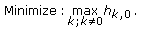 (45)
(45)
 ), the sidelobe levels must be reduced. This means that the total number of hits, given by
 . We know from the previous condition that the sum total of all the elements of
  over all values of
  equals
  . Also,
  is constant and is equal to
  . Our objective, therefore, is to spread out the remaining
  elements corresponding to
  peaks over the
  summation terms of
  (excluding
  ) thereby minimizing the peak sidelobe. This can be expressed in compact form as follows
6.1. Waveform Design
In this section, we propose a direct waveform design algorithm that yields codes that satisfy both Conditions A and B described above. This algorithm requires the number of frequencies  to be constrained to
  (the consequences of such a restriction are discussed in the next subsection).
Towards finding codes that satisfy Condition A, we define

Since  and
and  , we can write
  . Hence, minimizing
  for a given value of
  is equivalent to minimizing
  . Now, from (43) we note that if the pair of entries
  and
and  in the code matrix
  are equal, they will contribute a value of 1 (or one "hit") to
  at
at  . Thus we can say that
  will equal the number of pair of entries with identical values that can be found in the code matrix.
Using this alternate interpretation of  , we proceed to show that under the constraint
  ,
,  will be minimized only when each of the
  usable frequency values occur exactly twice in the code matrix. To see this, consider an example with
  , which means that the code matrix has 6 entries and 3 frequency choices are available. Let
  ,
,  and
and  correspond to the 3 frequencies. If we choose each of these three frequencies twice, that is, we make the selection
  , the possible pairs of entries with identical frequencies will be
  ,
,  and
and  , thus giving
  . Suppose we pick
  , the number of possible same-frequency pairs will be four: one
  pair and three
  pairs giving
  , one higher than the case where each frequency was used twice. Other combinations can also be shown to yield a higher value of
  . A similar argument can be extended to other values of
  and
and  as well.
Next, we provide the conditions under which Condition B will be satisfied. Any code matrix with  and with each frequency used twice will have
  . In order to satisfy Condition B, we require that these
  hits be spread as uniformly as possible among the
  summation terms of (46). This leads to the condition

where

which implies that all the values of  for
for  must equal either
  or
or  .
.
For a given value of  and
and  , there will exist several code matrices that satisfy Conditions A and B simultaneously. We now describe an algorithm that will randomly generate one such code matrix in each run. Initially, we start with a code matrix that has all entries "vacant", and hence
  for all
  . The algorithm has two steps. In Step 1 (see Figure 11), we first randomly select a pair of vacant entries
  and
and  such that
  , and fill these entries with frequency index 1. This increments the value of
  at
at  by 1, while leaving it unchanged for other values of
  . We repeat this procedure another
  times, using a different frequency index each time, until we have
  at
at  . Next we proceed to similarly increment the other values of
  to
to  , in the order
  . Step 1 is completed when
  at
at  .
.

Step 1 of the algorithm.
In the cases where  is not an integer, the code matrix will still have some vacant entries after Step 1. Step 2 of the algorithm (see Figure 12) aims to fill the remaining entries, while ensuring that

This is achieved by again traversing through the values of  in the order
  , and incrementing by one hit wherever possible. Flow charts providing the details of the two steps are shown in Figures 11 and 12. As can be seen from the algorithm flow charts, there are certain cases under which we need to discard the code matrix obtained after a few iterations and restart from the beginning of Step 1. This case arises when, from a partially filled code matrix, it is not possible to fill the remaining positions in such a way that the resulting code matrix will generate orthogonal waveforms. However, the probability of such an event occurring is very low. Through extensive simulations (for various values of
  and
and  ), we have observed that the probability of a code being generated with three or less restarts is over 99%.

Step 2 of the algorithm.
Consider a simple example for  and
and  . Since
  is not an integer, both Step 1 and Step 2 will need to be performed. The one possible sequence of code matrices obtained at various stages of the algorithm are shown in Figure 13.

A possible sequence of code matrices obtained at various stages of the algorithm ( and
and  ).
).
6.2. Related Discussion
For frequency-hopping waveforms, the parameters which can be controlled are -  . The proposed algorithm assumes one of these parameters
  to be equal to
  . One possible limitation of this method is the loss of flexibility in designing codes for a required time-bandwidth product,
  . Table 1 lists all possible time-bandwidth products between 0 and 400 for which codes can be designed from the proposed algorithm for
  . Note that the bandwidth of the waveform is
  , the duration of each pulse is
  and, hence,
  . From the entries of the table, we may state that constraint on
  is not a serious limitation on the flexibility in designing the code. On the other hand, the algorithm hardly needs any computations in comparison to those required by a heuristic search-based method such as simulated annealing.
 for which codes can be designed with the proposed algorithm (
 and
and  ).
).6.3. Simulation Results
We will now present simulation results to demonstrate the effectiveness of our proposed algorithm. We have generated codes of various sizes using both methods, the heuristic search proposed by [11] with the cost function (41) at  and our proposed algorithm. The code parameters used were
  ,
,  and
and  for each value of
  . From the code matrices obtained from both methods for
  ,
,  , we plotted the Empirical CDFs of their respective
  functions (see Figure 14). In order to see how a randomly generated code performs on average, we generated randomly 100 orthogonal code matrices of same size and plotted ECDF of the code corresponding to the median cost. Note from the plots that both methods are similar in terms of performance and they show a marked improvement over a randomly generated code.

Empirical CDFs of the codes from the two methods ( ,
,  , and
, and  ).
).
In order to compare the performance of the two methods with increasing code size, we have plotted the magnitude below which 95% of the samples of  lie. The lower the curve, the lower is the corresponding sidelobe level, which corresponds to a better code. From Figure 15, we see that the performance of the proposed algorithm is either very similar or slightly better than that of the heuristic search-based method for all
  . The marginal performance loss of the heuristic method for some values of
  , as seen in the figure, may be because the simulated annealing has converged to one of the local minima.

Magnitude of 95th percentile of  (
( ).
).
7. Weighted Optimization ( )
)
 )
)When optimizing frequency-hopping codes using either  and
and  , the aim is to minimize the sidelobe levels over the entire range of delay-Doppler space, that is, for
  and
and  . However, it is possible to place a higher importance on the minimization of sidelobe peaks in a subregion of the delay-Doppler space, by using a weighted cost function defined as follows:

where  is the weight applied to
  th element of
  (see (20)). We now discuss possible applications of such a weighted cost function.
Example 1.
When the range of target Doppler is smaller than the overall bandwidth of the transmitted signals ( ), optimization can be performed for a subset of the Doppler values using the weights:

where  .
.
Example 2.
Using this method, it is possible to find waveforms with their ambiguity sidelobes constrained to particular regions of the the delay-doppler space. Suppose we wish to find codes with very few ambiguity sidelobes occurring in a region close to the mainlobe. Consider the following mask

where  and
and  are bounds on the regions of delay-Doppler space. Thus, a penalty is applied on sidelobes occurring inside the region of interest and the cost is unaffected by sidelobes occurring outside this bounded region. To show the gain this method could have, we now compare the final ambiguity functions obtained by using
  and
and  . In order to compare them, we consider the delay-Doppler subspace of the corresponding ambiguity functions bounded by
  and
and  and plot their respective CDFs. The parameters for this simulation were
  ,
,  ,
,  ,
,  and
and  . Figure 16 shows the gain achievable within the region of interest.

CDFs of the optimized codes with and without weighting in the specified region ( ,
,  ,
,  ,
,  ,
,  ).
).
8. Conclusion
In this paper, we have shown how the MIMO radar ambiguity function for orthogonal frequency-hopping waveforms can be extended to general values of Doppler. We have also presented the hit-matrix as an analysis tool for these waveforms. To enable the optimization of these waveforms under the large Doppler scenario using simulated annealing, cost functions have been presented based on the ambiguity function as well as the hit-matrix. The codes obtained using both cost functions are shown to have similar performance based on their ECDF curves. The hit-matrix-based cost function has a significantly lower computational complexity, and can be useful when searching for codes with high time-bandwidth products, where using a ambiguity-based cost function is infeasible.
Under the small Doppler scenario, an algorithm has been proposed which directly computes the code matrix of a given size. It has been shown to perform as well as the heuristic search proposed by Chen and Vaidyanathan [11]. The use of weighted cost functions to optimize the ambiguity function within a subregion of the delay-Doppler space has also been explored. This method of "Weighted Optimization" also addresses the problem of waveform design for intermediate Doppler.
References
Fishler E, Haimovich A, Blum R, Chizhik D, Cimini L, Valenzuela R: MIMO radar: an idea whose time has come. Proceedings of the IEEE Radar Conference, April 2004 71-78.
Li J, Stoica P: MIMO radar with colocated antennas. IEEE Signal Processing Magazine 2007, 24(5):106-114.
Li J, Stoica P: MIMO Radar Signal Processing. Wiley-IEEE Press, New York, NY, USA; 2008.
Golomb SW: Constructions and properties of costas arrays. Proceedings of the IEEE 1984, 72(9):1143-1163.
Levanon N, Mozeson E: Radar Signals. Wiley-IEEE Press, New York, NY, USA; 2004.
Deng H: Discrete frequency-coding waveform design for netted radar systems. IEEE Signal Processing Letters 2004, 11(2):179-182. 10.1109/LSP.2003.821693
Liu B, He Z: Orthogonal discrete frequency-coding waveform design for MIMO radar. Journal of Electronics 2008, 25(4):471-476. 10.1007/s11767-007-0009-0
Bellegarda JR, Maric SV, Titlebaum E: The hit array: a synthesis tool for multiple access frequency hop signal. IEEE Transactions on Aerospace and Electronic Systems 1993, 29(3):624-635. 10.1109/7.220958
Bellegarda JR, Titlebaum EL: The hit array: an analysis formalism for multiple access frequency hop coding. IEEE Transactions on Aerospace and Electronic Systems 1991, 27(1):30-39. 10.1109/7.68145
Chen C-Y, Vaidyanathan PP: Properties of the MIMO radar ambiguity function. Proceedings of the IEEE International Conference on Acoustics, Speech and Signal Processing (ICASSP '08), April 2008 2309-2312.
Chen C-Y, Vaidyanathan PP: MIMO radar ambiguity properties and optimization using frequency-hopping waveforms. IEEE Transactions on Signal Processing 2008, 56(12):5926-5936.
San Antonio G, Fuhrmann DR, Robey FC: MIMO radar ambiguity functions. IEEE Journal on Selected Topics in Signal Processing 2007, 1(1):167-177.
Acknowledgments
The authors gratefully acknowledge the useful comments and suggestions of the reviewers which improved the clarity of the paper. One of the authors, V. U. Reddy, wishes to acknowledge the partial support he received from CR Rao Advanced Institute of Mathematics, Statistics and Computer Science for this work.
Author information
Authors and Affiliations
Corresponding author
Rights and permissions
Open Access This article is distributed under the terms of the Creative Commons Attribution 2.0 International License ( https://creativecommons.org/licenses/by/2.0 ), which permits unrestricted use, distribution, and reproduction in any medium, provided the original work is properly cited.
About this article
Cite this article
S, B., Srinivas, A. & Reddy, V.U. Low-Complexity Design of Frequency-Hopping Codes for MIMO Radar for Arbitrary Doppler. EURASIP J. Adv. Signal Process. 2010, 319065 (2010). https://doi.org/10.1155/2010/319065
Received:
Revised:
Accepted:
Published:
DOI: https://doi.org/10.1155/2010/319065