Hierarchical CoSaMP for compressively sampled sparse signals with nested structure

Abstract

This paper presents a novel procedure, named Hierarchical Compressive Sampling Matching Pursuit (CoSaMP), for reconstruction of compressively sampled sparse signals whose coefficients are organized according to a nested structure. The Hierarchical CoSaMP is inspired by the CoSaMP algorithm, and it is based on a suitable hierarchical extension of the support over which the compressively sampled signal is reconstructed. We analytically demonstrate the convergence of the Hierarchical CoSaMP and show by numerical simulations that the Hierarchical CoSaMP outperforms state-of-the-art algorithms in terms of accuracy for a given number of measurements at a restrained computational complexity.

1 Introduction

The burgeoning field of compressive sampling (CS) addresses the recovery of signals which are sparse either in the original domain or in a different representation domain achieved by a suitable invertible transform. The CS theory establishes conditions for sparse signals recovering from measurements acquired without satisfying the Nyquist criterion, provided that suitable relations between the number of measurements and the signal sparsity are satisfied. CS studies encompass different issues, ranging from measurement acquisition via random projections to signal recovery algorithms; besides, CS reconstruction algorithms possibly leverage specific signals underlying structure. The reconstruction algorithm Compressive Sampling Matching Pursuit (CoSaMP) by Needell and Tropp [1] represents a starting point in the definition of reconstruction procedures. The reason is manifold. Firstly, its solid analytical derivation is viable of different extensions accounting for peculiar signal structures [2]. Secondly, its iterative structure may be extended to encompass prior knowledge on the signal to be reconstructed [3]. Besides, the CoSaMP gracefully degrades with noise, since the reconstruction error is bounded by a value proportional to the energy of the noise vector, for a sufficiently large number of measurements.

In principle, the minimal number of measurements for the CoSaMP algorithm to converge on sparse noise-free signal is the least required by CS theory [1]. Still, in [4], it is observed that procedures exploiting the sparse signal structure can converge with a number of measurements of the order of the signal sparsity [5], whereas numerical examples show that the CoSaMP may require a number of measurements about four times larger than the signal sparsity. Thereby, it is argued that in specific applications, the number of measurements may be in principle sufficient to recover the signal under concern, exactly or in an approximate form, while still not being enough for the CoSaMP to converge. This limits the accuracy and applicability of CoSaMP in a variety of resource-limited applications, such as CS in sensor networks [6].

Several studies have been so far proposed to overcome the gap between the minimum number of measurements as predicted by CS theory and those required by the CoSaMP to converge. A fundamental study by Baraniuk et al. [2] proposes to exploit knowledge about peculiar structures exhibited by the sparse signal. Specifically, the authors focus on the reconstruction of K-compressible signals, e.g. signals that are approximately reconstructed by K coefficients, and show that if the signal presents a suitable structure, the reconstruction procedure can exploit this knowledge to constrain the recovered signal subspace and improve the accuracy for a given number of measurements.

The analysis in [2] introduces the concept of nested approximation property of a signal sparsity model to derive theoretical bounds for CS reconstruction. Further, a priori constraints on the structure of the compressible signal, e.g. the organization in blocks or in a tree structure, are then invoked to take advantage of the signal sparsity model and reduce the solution space of the recovery algorithm.

Herein, in the light of the work in [2], we concern ourselves with signals whose coefficients are organized according to a nested structure. For such signals, we introduce a modified version of the CoSaMP algorithm, referred to as Hierarchical CoSaMP (HCoSaMP), that exploits the underlying assumption that the signal is hierarchically structured. Specifically, in HCoSaMP, the estimated support is progressively extended from a hierarchical layer to another throughout different estimation stages. Different from the analysis in [2], only the assumption on the nested signal structure is needed to formally state the convergence of the HCoSaMP. Thereby, the herein presented analysis imposes mild assumptions on the signals, and it applies in general cases where structured sparsity cannot be claimed. Besides, we provide application examples on images obtained by oceanographic monitoring [6, 7] and natural images [8], as well as on texture images [9]. For the former cases, we select the well-known discrete wavelet transform as a sparsifying transform, whereas for the latter, we resort to the graph-based transform, originally established for depth map encoding, as a sparsity-achieving representation within the reconstruction procedure. In both cases, we show that our procedure outperforms state-of-the-art reconstruction algorithms and proves extending the feasibility of the reconstruction in the presence of a reduced number of measurements.

The structure of the paper is as follows. In Section 2, we recall the CS basics, while in Section 3, we discuss the CS of a sparse signal with nested structure. In Section 4, we describe the HCoSaMP and outline the demonstration of its convergence, and in Section 5, we report the numerical simulation results. Finally, Section 6 concludes the paper.

2 Compressive sampling basics

Let us consider an image x[n₁,n₂], and let us denote by x the N×1 vector built by collecting its samples in lexicographic order; besides, let us assume that x is K-sparse. Let y denote the M×1 vector of CS measurements, given by

$$\mathbf{y}=\tilde{\mathit{\Phi }}\mathbf{x}+\mathbf{n}$$

(1)

where $\tilde{\mathit{\Phi }}$ is a suitable M×N random sensing matrix, and n is the M×1 acquisition noise. For perfect reconstruction of x given y, the sensing matrix $\tilde{\mathit{\Phi }}$ is supposed to satisfy the restricted isometry property (RIP) [10]:

$$(1-{\delta }_K)\parallel \mathbf{x}{\parallel }_2^2\le \parallel \tilde{\mathit{\Phi }}\mathbf{x}{\parallel }_2^2\le (1+{\delta }_K)\parallel \mathbf{x}{\parallel }_2^2.$$

(2)

It can be proved that a matrix $\tilde{\mathit{\Phi }}$ with i.i.d. random entries drawn from a Gaussian distribution with zero mean and variance 1/M satisfies the RIP with high probability [11, 12] provided that

$$M\ge M_K=C_m\frac{Klog(N/K)}{{\delta }_K^2}.$$

(3)

Similar results have been derived for different classes of random sensing matrices. The relation (3) binds the signal sparsity K and the minimal number of measurement M _K for the matrix $\tilde{\mathit{\Phi }}$ to obey the RIP with a given RIP constant value δ _K ; conversely, for a K-sparse signal, the RIP constant value δ _K with which a selected matrix $\tilde{\mathit{\Phi }}$ satisfies the RIP depends on the available number of measurements M (see [13] for a detailed discussion), and being fixed the value of M, the value of δ _k increases with K.

Often, the signal is assumed to be sparse under a sparsifying transformation identified by a transform basis matrix Ψ. Then, x is expressed as x=Ψ α where the vector α collects the transform coefficients and it is defined on a set$\mathbb{L}$ of cardinality $\left|\mathbb{L}\right|=N$. With these positions, and because of the decomposition in (5), we can rewrite the acquisition process in (1) via a sensing matrix $\mathit{\Phi }\stackrel{\text{def}}{=}\tilde{\mathit{\Phi }}\mathit{\Psi }$ as follows:

$$\mathbf{y}=\mathit{\Phi }\mathbf{\alpha }+\mathbf{n}.$$

(4)

In the following, we refer to a K-sparse signal such that only K out of its N transform coefficients are non-zero valued; besides, we denote by Ω the support of the K non-zero coefficients of α, satisfying $\Omega \subseteq \mathbb{L}$ and having cardinality |Ω|=K<N.

3 CS of a sparse signal with nested structure

Let us consider a group of L+1 subsets ${\mathbb{L}}_i,i=0,\dots ,L$ of the overall set$\mathbb{L}$, such that ${\mathbb{L}}_0\subset {\mathbb{L}}_1\subset \dots {\mathbb{L}}_L=\mathbb{L}$. We also consider a partition of the support Ω of the non-zero terms of α into a finite number of sets Ω _l ,l=0,…,L of cardinality K _l =∥Ω _l ∥,l=0,…,L, defined as follows:

$$\begin{array}{ll}{\Omega }_0& =\Omega \cap {\mathbb{L}}_0,\\ {\Omega }_l& =\left(\Omega \cap {\mathbb{L}}_l\right)\setminus {\Omega }_{l-1},l=1,\dots ,\mathrm{L.}\end{array}$$

The sets Ω _i ’s are disjoint, i.e. Ω _i ∩Ω _j =⊘,j≠i and the union of the Ω _i ’s up to the L-th, is ${\cup }_{i=0}^L{\Omega }_i=\Omega$.

The above partition is found, for instance, in the L decomposition levels of the wavelet transform of a natural image, where the set ${\mathbb{L}}_0$ can be associated to the indexes of the scaling coefficients, and the sets ${\mathbb{L}}_l,l=1,\dots ,L$ can be formed by progressively including the indexes corresponding to the increasing wavelet decomposition levels. In this example, the set ${\Omega }_0=\Omega \cap {\mathbb{L}}_0$ is built by the indexes of the non-zero scaling coefficients, and the sets Ω _l ,l=1,…,L correspond to the incremental supports of the non-zero coefficients found in each of the ${\mathbb{L}}_l$’s. Although the most familiar, the wavelet domain is not the sole one in which a hierarchical organization of the transform coefficients is observed. In Section 5, we show with the help of numerical examples that the graph-based transform (GBT) transform of texture images reveals a hierarchical structure, too.

The signal x satisfies the nested approximation property (NAP) if the support of the best (in the least squares sense) K-term approximation in ${\mathbb{L}}_i$ includes the support of the best K^′-term approximation in ${\mathbb{L}}_{i-1}$ for all K≥K^′, and for i=1,…L. This property, referred to as the NAP, is invoked in [2] on structured sparse signal models to derive a tight bound on the number of CS measurements required for signal reconstruction. The therein presented recovery algorithm exploits a priori knowledge on the structured nature of the signal. Herein, we drop further hypotheses on the signal structure, and we elaborate on the nestedness of the signal support.

Let us then consider a signal x represented by a sparsifying transform Ψ, and let us assume that it satisfies the NAP in the transform domain. We rewrite the vector α as $\mathbf{\alpha }=\sum _l{\mathbf{\alpha }}_{{\Omega }_l}$, where ${\mathbf{\alpha }}_{{\Omega }_l}$ denotes a vector whose entries coincide with α for indexes in Ω _l and are zero otherwise. Each subset ${\mathbf{\alpha }}_{{\Omega }_l}$ of the elements of α has sparsity K _l , and the union of the Ω _i ’s up to the l-th, namely ${\cup }_{\lambda =0}^l{\Omega }_{\lambda }$, of cardinality $K_l=\sum _{\lambda =0}^l{K}_{\lambda }$, yields the best K _l -term approximation of the signal itself.

The vector x can then be expressed as the sum of the contributions due to the different transform domain layers

$$\mathbf{x}=\mathit{\Psi }\sum _l{\mathbf{\alpha }}_{{\Omega }_l}=\sum _l{\mathit{\Psi }}_{{\Omega }_l}{\mathbf{\alpha }}_{{\Omega }_l}$$

(5)

where ${\mathit{\Psi }}_{{\Omega }_l}$ denotes the restriction of Ψ to the column indices of Ψ pertaining to different disjoint sets Ω _l .

Because of the decomposition in (5), we can rewrite the acquisition process in (4) as follows:

$$\mathbf{y}=\sum _l\mathit{\Phi }{\mathbf{\alpha }}_{{\Omega }_l}+\mathbf{n}.$$

(6)

For simplicity sake, and without loss of generality, let us first refer to a nested decomposition encompassing only two layers, i.e. l={0,1}. Under this position, we can rewrite (6) as

$$\mathbf{y}=\mathit{\Phi }{\mathbf{\alpha }}_{{\Omega }_0}+\mathit{\Phi }{\mathbf{\alpha }}_{{\Omega }_1}+\mathbf{n}=\mathit{\Phi }{\mathbf{\alpha }}_{{\Omega }_0}+{\mathbf{e}}_0.$$

(7)

The formulation in (7) gives a simple and yet interesting insight on the CS acquisition process. To elaborate, the M measurements collected in (7) can be interpreted as either (i) the acquisition of the K-sparse vector α with a measurement noise n of energy ∥n∥₂ or (ii) the acquisition of the K₀-sparse vector ${\mathbf{\alpha }}_{{\Omega }_0}$ with a measurement noise e₀ of energy ∥e₀∥₂, suitably bounded^a because of the RIP of the matrix Φ.

4 Hierarchical CoSaMP

Here, we propose a modified version of the CoSaMP procedure for reconstructing sparse signals exhibiting the above introduced nested structure. In short, we show that a signal endowed by such nested hierarchical structure can be reconstructed by recursive application of the core stage of the CoSaMP algorithm on progressively expanded supports. Furthermore, we show that the resulting procedure, which we refer to as Hierarchical CoSaMP (HCoSaMP), requires a lower number of measurements than the original CoSaMP to incrementally reconstruct the signal up to its best K-term approximation.

Before turning to mathematics, we make two observations. Firstly, the reformulation (7) of the relation in (6) hints to recover the coefficients of ${\mathbf{\alpha }}_{{\Omega }_0}$ starting from the measurements y, instead of trying to recover the whole signal α. The requirement on the number of measurements for the CoSaMP convergence in reconstructing the K₀ samples of ${\mathbf{\alpha }}_{{\Omega }_0}$ is indeed looser than that for reconstruction of the K samples of α _Ω . Specifically, the number M must satisfy the RIP for ${\delta }_{4K_0}$ but not for δ_4K[1]. If the RIP for ${\delta }_{4K_0}$ is satisfied, the samples ${\mathbf{\alpha }}_{{\Omega }_0}$ can be recovered by the CoSaMP algorithm [2] and numerical bounds relating the estimation error to the signal energy out of Ω₀ are provided.

Specifically, in [1], the accuracy achieved at convergence by the CoSaMP algorithm is characterized by the following mean square error bound:

$$\parallel \mathbf{\alpha }-{\mathbf{\alpha }}_{{\Omega }_0}{\parallel }_2\le 15\left(1.1\parallel \sum _l{\mathbf{\alpha }}_{{\Omega }_l}{\parallel }_2+\parallel \mathbf{n}{\parallel }_2\right).$$

(8)

From (8), we recognize that the performance of such CoSaMP-based stage degrades gracefully as the energy out of Ω₀ increases, just as it occurs when CoSaMP recovers noisy signals or compressible signals.

Secondly, let us assume to have recovered, to a certain degree of accuracy, the samples ${\mathbf{\alpha }}_{{\Omega }_0}$ starting from the measurements collected as in (7), so as to have the best K₀-term approximation of the sparse signal α. Then, this coarse estimate can be adopted as a better initialization of a CoSaMP procedure, in order to recover the remaining K₁ − K₀ coefficients providing the best K₁-term approximation of the α itself.

Stemming on these observations, it is fair to ask if the recovery of the signal on the l-th support can exploit the partial knowledge of the signal on the supports up to the (l−1)-th one. In the following subsection, we prove that if the signal under concern satisfies the NAP property, it is indeed possible to recover all the coefficients α by (i) first recovering the coefficients ${\mathbf{\alpha }}_{{\Omega }_0}$ and then (ii) recursively injecting the coefficients recovered on the support Ω_l−1 as initialization for recovering the coefficients ${\mathbf{\alpha }}_{{\Omega }_l}$ on the support Ω _l .

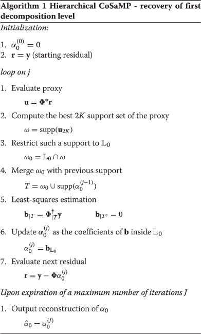
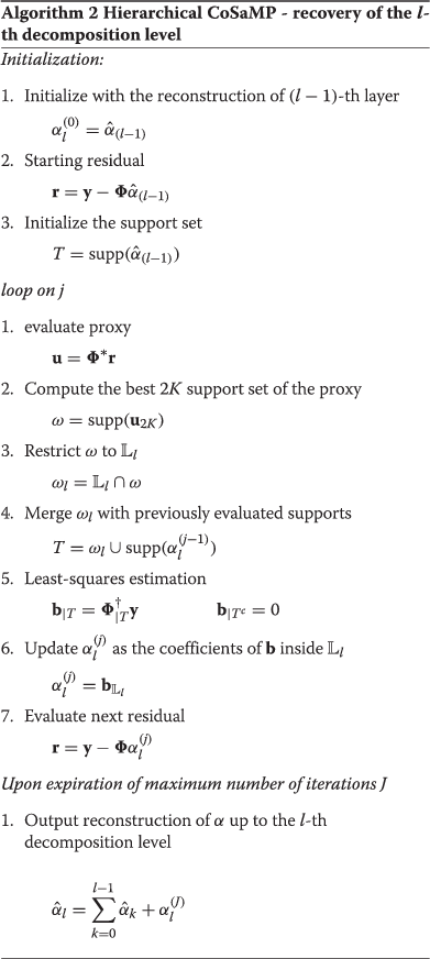
The recovery stages (i) and (ii) are respectively realized according to Algorithms 1 and 2, where we denote by Φ^† the pseudo-inverse of Φ, i.e. (Φ^∗Φ)⁻¹Φ^∗; by x _N the restriction of x to its N largest-magnitude components; by x_|T (A_|T) the restriction of x (A) to the elements (columns) of indices in the set T; and by |T| the cardinality of the set T.

To sum up, the outline of the HCoSaMP is as follows:

• (a) Recovery of the first decomposition layer. The outline of this partial estimation stage appears in Algorithm 1; this stage encompasses all the steps of the CoSaMP, plus an additional step (namely step 3 in Algorithm 1, which tailors the support estimated at each iteration to the predefined support ${\mathbb{L}}_0$.

• (b) Recovery of the l-th decomposition layer. The outline of the estimation stage providing the reconstruction of the signal up to the support Ω _l given its previous estimate up to the support Ω_l−1 appears in Algorithm 2. We recognize that this stage still reproduces the steps encompassed by the CoSaMP from which it differs because it is initialized with the reconstructed version of ${\mathbf{\alpha }}_{{\Omega }_{l-1}}$ and it limits the estimate to the support ${\cup }_{\lambda =0}^l{\Omega }_{\lambda }$.

  
  

In the following subsection, we formally prove the convergence of the HCoSaMP algorithm on NAP signals.

4.1 HCoSaMP convergence on a sparse signal with nested structure

The convergence theorem is presented in two parts, respectively establishing the convergence in Algorithm 1 (Part I) and in Algorithm 2 (Part II).

Theorem 4.1 (Part I: Convergence of Algorithm 1)

Let us consider ${\mathbf{\alpha }}_0\in {\mathbb{L}}_0$ with ${\mathcal{ℒ}}_0=\left|{\mathbb{L}}_0\right|$, and a set of M CS noisy measurements y obtained as y=Φ α₀+e₀ according to (7). If Φ exhibits a RIP constant ${\delta }_{{\mathcal{ℒ}}_0}\le 0.1$ for the value of M at hand, then it can be proved that the mean square error on the estimate ${\mathbf{\alpha }}_0^{\left(j\right)}$ obtained at the j-th iteration of the HCoSaMP algorithm can be upper bounded as follows:

$$\parallel {\mathbf{\alpha }}_0-{\mathbf{\alpha }}_0^{\left(j\right)}{\parallel }_2\le 4^{-j}\parallel {\mathbf{\alpha }}_0{\parallel }_2+15\parallel {\mathbf{e}}_0{\parallel }_2.$$

(9)

Proof

(Proof of Theorem 4.1, Part I) To prove the convergence of Algorithm 1, we follow the guidelines in [1], by adapting them to the nested signal structure invoked by the Hierarchical CoSaMP algorithm. Specifically, we show that the reconstruction error at the j-th iteration of the algorithm

$$\parallel {\mathbf{\alpha }}_0-{\mathbf{\alpha }}_0^{\left(j\right)}{\parallel }_2$$

(10)

is upper bounded by a term that, in the case of noise-free acquisition, decays asymptotically to zero. Towards this aim, we prove a series of inequalities providing the desired result.

At each iteration of the algorithm, the reconstructed signal ${\mathbf{\alpha }}_0^{\left(j\right)}$ is selected as the restriction of the least squares estimate b over the support ${\mathbb{L}}_0$. Based on such a restriction, considering that α₀ lives, by definition, over the support ${\mathbb{L}}_0$, we can write

$$\parallel {\mathbf{\alpha }}_0-{\mathbf{\alpha }}_0^{\left(j\right)}{\parallel }_2=\parallel {\mathbf{\alpha }}_0-{\mathbf{b}}_{{\mathbb{L}}_0}{\parallel }_2\le \parallel {\mathbf{\alpha }}_0-\mathbf{b}{\parallel }_2.$$

(11)

The following Lemma 4.1 provides an upper bound over the right-hand side of (11), representing the energy of the error of the least squares estimation in Algorithm 1.

Lemma 4.1

Let us consider the set T estimated as in Algorithm 1, and let b represent the LS estimate of the signal samples evaluated on the support T:

$$\begin{array}{l}{\mathbf{b}}_{|T}={\mathit{\Phi }}_{|T}^{†}\mathbf{y}={\mathit{\Phi }}_{|T}^{†}(\mathit{\Phi }{\mathbf{\alpha }}_0+{\mathbf{e}}_0)\\ {\mathbf{b}}_{|T^C}=\mathbf{0}\end{array}.$$

(12)

The energy of the estimation error is upper bounded by a term proportional to the energy of the signal α₀ over the support T^C and by a term proportional to the measurement noise energy:

$$\parallel {\mathbf{\alpha }}_0-\mathbf{b}{\parallel }_2\le \parallel {\mathbf{\alpha }}_{0|T^C}\parallel \left(1+\frac{{\delta }_{{\mathcal{ℒ}}_0}}{1-{\delta }_{{\mathcal{ℒ}}_0}}\right)+\frac{\parallel {\mathbf{e}}_0\parallel }{\sqrt{1-{\delta }_{{\mathcal{ℒ}}_0}}}.$$

(13)

The proof of Lemma 4.1 is found in Appendix 1.

We recognize that the term $\parallel {\mathbf{\alpha }}_{0|T^C}\parallel$ in (13) represents the energy of the original signal ${\mathbf{\alpha }}_{0|T^C}$ outside the set T. Since ${\mathbf{\alpha }}_0^{\left(j\right)}$ has no energy over T^C, we can write

$$\parallel {\mathbf{\alpha }}_{0|T^C}\parallel =\parallel {({\mathbf{\alpha }}_0-{\mathbf{\alpha }}_0^{\left(j\right)})}_{|T^C}\parallel .$$

(14)

In turn, the energy of the error is upper bounded by the energy of the signal to be recovered at iteration j over the set ω₀^C, that is with the energy

$$\parallel {({\mathbf{\alpha }}_0-{\mathbf{\alpha }}_0^{\left(j\right)})}_{|T^C}\parallel \le \parallel {({\mathbf{\alpha }}_0-{\mathbf{\alpha }}_0^{\left(j\right)})}_{|{{\omega }_0}^C}\parallel .$$

(15)

In order to upper bound this latter term, we resort to the following Lemma 4.2, whose proof can be found in Appendix 2.

Lemma 4.2

Let α be a K-sparse signal with support$\mathbb{L}$ and α₀ be the portion of α confined to the support ${\mathbb{L}}_0\subset \mathbb{L}$, of cardinality ${\mathcal{ℒ}}_0$. Under these settings, the estimate of the vector α₀ obtained after the j-th iteration of the HCoSaMP algorithm, namely ${\mathbf{\alpha }}_0^{\left(j\right)}$, is the same as that obtained by application of the CoSaMP, with the following positions:

$$\begin{array}{ll}\hfill \mathbf{s}& ={\mathbf{\alpha }}_0-{\mathbf{\alpha }}_0^{\left(j\right)}\left(\mathit{\text{Signal}}\mathit{\text{not}}\mathit{\text{yet}}\mathit{\text{recovered}}\mathit{\text{at}}\mathit{\text{iteration}}j\right)\\ \hfill \mathbf{r}& =\mathbf{y}-\mathit{\Phi }{\mathbf{\alpha }}_0^{\left(j\right)}=\mathit{\Phi }\mathbf{s}+{\mathbf{e}}_0(\mathit{\text{Residual}}\mathit{\text{at}}\mathit{\text{iteration}}j-\mathit{\text{it}}\mathit{\text{is}}\\ \mathit{\text{just}}a\mathit{\text{CS}}\mathit{\text{acquisition}}\mathit{\text{of}}\mathit{\text{the}}\mathit{\text{signal}}\mathbf{s})\\ \hfill \mathbf{u}& ={\mathit{\Phi }}^{\ast }\mathbf{r}\left(\mathit{\text{Proxy}}\mathit{\text{at}}\mathit{\text{iteration}}j\right)\\ \hfill {\omega }_0& ={\mathbb{L}}_0\cap \text{supp}\left({\mathbf{u}}_{2K}\right)\end{array}$$

(16)

where the term e₀ encompasses not only acquisition noise but also approximation error on the support ${\mathbb{L}}_0$. It can then be proved that:

$$\begin{array}{cc}\parallel {({\mathbf{\alpha }}_0-{\mathbf{\alpha }}_0^{\left(j\right)})}_{|{{\omega }_0}^C}{\parallel }_2& \le \frac{2{\delta }_{{\mathcal{ℒ}}_0}\parallel {\mathbf{\alpha }}_0-{\mathbf{\alpha }}_0^{\left(j\right)}{\parallel }_2+2\sqrt{1+{\delta }_{{\mathcal{ℒ}}_0}}\parallel {\mathbf{e}}_0{\parallel }_2}{(1-{\delta }_{{\mathcal{ℒ}}_0})}.\end{array}$$

(17)

The result expressed by (17) shows that when the algorithm selects the support ω₀ from the proxy at iteration j, it is able to identify most of the energy of the portion of the signal that still has to be recovered at iteration j.

Injecting (14), (15) and (17) in (13), we finally come up with the desired upper bound to the reconstruction error energy

$$\begin{array}{ll}\hfill \parallel {\mathbf{\alpha }}_0-{\mathbf{\alpha }}_0^{\left(j\right)}{\parallel }_2\le & \left(\frac{2{\delta }_{{\mathcal{ℒ}}_0}\parallel ({\mathbf{\alpha }}_0-{\mathbf{\alpha }}_0^{\left(j\right)}){\parallel }_2+2\sqrt{1+{\delta }_{{\mathcal{ℒ}}_0}}\parallel {\mathbf{e}}_0{\parallel }_2}{(1-{\delta }_{{\mathcal{ℒ}}_0})}\right)\\ \times \left(1+\frac{{\delta }_{{\mathcal{ℒ}}_0}}{1-{\delta }_{{\mathcal{ℒ}}_0}}\right)+\frac{\parallel {\mathbf{e}}_0\parallel }{\sqrt{1-{\delta }_{{\mathcal{ℒ}}_0}}}.\end{array}$$

(18)

By setting, as in [1, 2], ${\delta }_{{\mathcal{ℒ}}_0}\le 0.1$, we can rewrite (18) as

$$\parallel {\mathbf{\alpha }}_0-{\mathbf{\alpha }}_0^{\left(j\right)}{\parallel }_2\le 0.25\parallel {\mathbf{\alpha }}_0-{\mathbf{\alpha }}_0^{\left(j\right)}\parallel +3.6\parallel {\mathbf{e}}_0{\parallel }_2$$

which, solving the recursion, resolves in the expression in (9)

$$\parallel {\mathbf{\alpha }}_0-{\mathbf{\alpha }}_0^{\left(j\right)}{\parallel }_2\le 4^{-j}\parallel {\mathbf{\alpha }}_0{\parallel }_2+15\parallel {\mathbf{e}}_0{\parallel }_2.$$

(19)

Having proved the convergence of Algorithm 1, we proceed to discuss the convergence of Algorithm 2, devoted to the reconstruction of the i-th decomposition layer.

Theorem 4.1 (Part II: Convergence of Algorithm 2)

Let us assume to have recovered an estimate ${\widehat{\mathbf{\alpha }}}_{(i-1)}$ of the original signal α_(i−1). Then, it can be proved that the signal ${\mathbf{\alpha }}_i\in {\mathbb{L}}_i$ with ${\mathcal{ℒ}}_i=\left|{\mathbb{L}}_i\right|$ can be recovered at the j-th iteration of the HCoSaMP algorithm with a mean squared error bounded by

$$\parallel {\mathbf{\alpha }}_i-{\mathbf{\alpha }}_i^{\left(j\right)}{\parallel }_2\le 4^{-j}\parallel {\mathbf{\alpha }}_i{\parallel }_2+15\parallel {\mathbf{e}}_i{\parallel }_2$$

(20)

provided that the sensing matrix exhibits a RIP constant ${\delta }_{{\mathcal{ℒ}}_i}\le 0.1$.

Proof.

(Proof of Theorem 4.1, Part II) We restrict ourselves, for the sake of concreteness, to the case of a two-layer decomposition, i.e. α=α₀+α₁. The extension to the case of multiple decomposition layers is straightforward.

Let us then assume that the signal α₀ has been correctly recovered by running Algorithm 1; upon convergence, the reconstructed signal can be written as

$${\widehat{\mathbf{\alpha }}}_0={\mathbf{\alpha }}_0+{\mathbf{n}}_0$$

(21)

where the noise term n₀ accounts for both convergence inaccuracies due to a finite number of iterations and the error floor due to the presence of the acquisition noise. Algorithm 2 aims at recovering the signal α₁. The algorithm starts by initializing the output at the first iteration with the reconstructed version of α₀, that is

$${\mathbf{\alpha }}_1^{\left(0\right)}={\widehat{\mathbf{\alpha }}}_0.$$

Under this setting, the starting residual rewrites as follows:

$$\begin{array}{ll}\hfill \mathbf{r}& =\mathbf{y}-\mathit{\Phi }{\widehat{\mathbf{\alpha }}}_0\\ =\mathit{\Phi }({\mathbf{\alpha }}_0+{\mathbf{\alpha }}_1)+\mathbf{n}-\mathit{\Phi }({\mathbf{\alpha }}_0+{\mathbf{n}}_0)\\ =\mathit{\Phi }{\mathbf{\alpha }}_1+{\mathbf{e}}_1\end{array}$$

(22)

where we have compactly denoted e₁=n−Φ n₀. The relation in (22) shows that the selected initialization makes Algorithm 2 equivalent to the execution of Algorithm 1 aimed at recovering α₁ with a null initialization. Hence, following the steps in the proof of Part I,

we obtain

$$\parallel {\mathbf{\alpha }}_1-\mathbf{b}{\parallel }_2\le \parallel {\mathbf{\alpha }}_{1|T^C}\parallel \left(1+\frac{{\delta }_{{\mathcal{ℒ}}_1}}{1-{\delta }_{{\mathcal{ℒ}}_1}}\right)+\frac{\parallel {\mathbf{e}}_1\parallel }{\sqrt{1-{\delta }_{{\mathcal{ℒ}}_1}}}$$

(23)

where the set T now assumes a cardinality $\left|T\right|\le {\mathcal{ℒ}}_1$.

Let us now rephrase the positions in (16) as follows:

$$\begin{array}{ll}\mathbf{s}& ={\mathbf{\alpha }}_1-{\mathbf{\alpha }}_1^{\left(j\right)}\text{(Signal not yet recovered at iteration}j\text{)}\\ \mathbf{r}& =\mathbf{y}-\mathit{\Phi }{\mathbf{\alpha }}_1^{\left(j\right)}=\mathit{\Phi }\mathbf{s}+{\mathbf{e}}_1;\text{(Residual at iteration}j\text{- it is}\\ \text{just a CS acquisition of the signal}\mathbf{s}\text{)}\\ \mathbf{u}& ={\mathit{\Phi }}^{\ast }\mathbf{r}\\ {\omega }_1& ={\mathbb{L}}_1\cap \text{supp}\left({\mathbf{u}}_{2K}\right)\end{array}$$

In this case, s is confined to ${\mathbb{L}}_1$ so that its sparsity is bounded by ${\mathcal{ℒ}}_1=\left|{\mathbb{L}}_1\right|$. Then, stemming from the NAP property we can write

$$\parallel \mathbf{u}-{\mathbf{u}}_{|{\omega }_1}{\parallel }_2^2\le \parallel \mathbf{u}-{\mathbf{u}}_{\left|\text{supp}\right(\mathbf{s})}{\parallel }_2^2.$$

(24)

Then, following the same derivations driving to (17), we come up with the following inequality

$$\parallel {\mathbf{s}}_{|{{\omega }_1}^C}{\parallel }_2\le \frac{2{\delta }_{{\mathcal{ℒ}}_1}\parallel {\mathbf{\alpha }}_1-{\mathbf{\alpha }}_1^{\left(j\right)}{\parallel }_2+2\sqrt{1+{\delta }_{{\mathcal{ℒ}}_1}}\parallel {\mathbf{e}}_1{\parallel }_2}{(1-{\delta }_{{\mathcal{ℒ}}_1})}.$$

(25)

With this rephrasing, the overall convergence of Algorithm 2 is proved according to the derivations already exposed in Part I.

From the computational complexity point of view, with respect to the original CoSaMP and to its adaptation to the structured signal in [2], the HCoSaMP just exploits the layered structure of the image transform and requires L+1 applications of the basic stage; the latter in turn retains the computational complexity of the CoSaMP.

4.2 Related works

With respect to [2], the HCoSaMP poses milder assumptions since it does not invoke any constraint on the structure (e.g. tree-based, block-based) of the sparse signal. Still, as shown in the next section, the HCoSaMP achieves reconstruction accuracy performances comparable to that achieved by CS recovery with a larger number of measurements. In a nutshell, the reason is to be found in that the hierarchical approach allows each stage of the reconstruction algorithm to separately recover signal components on supports Ω _l whose cardinality K _l is smaller than that of the signal, i.e. K _l <K; the increased ratio between the number of measurements M and the sparsity K _l of the signal to be actually recovered definitely improves the convergence conditions. This capability is a merit of the HCoSaMP that leverages the nested signal structure that can be found in different domains depending on the application under concern.

The problem of the convergence of greedy algorithms on different subsets of the sparsity domain is debated in [14], where the authors focus on the CS recovery algorithm stability. The algorithm stability is said to be locally nested if the algorithm convergence on an outer set implies the convergence in all the inner subsets. In [14], it is shown that this property does not pertain to several greedy algorithms for CS recovery. Thereby, in the absence of assumptions on the nested structure of the signal, the algorithm convergence does not propagate from the more comprehensive set to the inner subsets. In our analysis, we instead prove the convergence on the entire domain by proving the convergence on a selection of hierarchically organized nested subsets, starting from the inner one up to the outer one.

A relevant question naturally arises about how to select the nested subsets. The first step is indeed the identification of a domain in which the signal is either sparse or compressible. Once the sparsity domain is identified, the second step is in partitioning the coefficients into nested subsets; in the sparsity domain, the support nesting often naturally arises when the signal energy is much more concentrated in lower frequency subsets and it decreases towards higher frequency subsets. This is the case of natural images, which typically are sparse and nested in the discrete wavelet transform (DWT) domain. A second example is found in video compressive sensing, where nested approximation may be invoked when the video data is suitably transformed in a 3D discrete cosine transform domain [15]. In the following, we show with the help of numerical examples that also texture images verify the NAP in the graph-based transform (GBT) [16] domain. Once a layered support structure allows to invoke the NAP on the signal under concern, the size of each set Ω _l ,l = 0,…L−1 shall be assigned according to a fundamental trade-off: smaller cardinality sets have looser CS measurement requirements but may result into slower convergence characteristics in case of high out-of-band energy. Henceforth, the choice of the subset cardinality depends on application-related issues, such as the acquisition noise level or the cost of the measurement acquisition stage.

Moreover, in general, the acquisition phase itself could in principle be designed so as to reduce the approximation error on the inner nested subsets, by organizing the sensing matrix so as to relate subsets of the measurements to subsets of the signal sparsity domain, much in the same way as block diagonal matrices [17, 18]; further analysis is needed to investigate on the RIP of a CS matrix inducing a nested structure on the acquired CS measurements.

Finally, the herein presented analysis draws a path for hierarchical solution of different recovery algorithms, such as the total variation minimization, which have been proved effective in video CS applications [15]. Recent literature results [19] have shown that the total variation (TV) minimization algorithm is guaranteed to converge also in the presence of acquisition noise. This paves the way to hierarchical application of the TV algorithm to progressively extended nested sets, on which the approximation error plays just the same role as the acquisition noise. The extension of the hierarchical approach to TV minimization is left for further study.

5 Numerical simulation

We now present numerical results assessing the performance of HCoSaMP in reconstructing signals characterized by the NAP; we both investigate the case of signals compressible in the DWT domain and the interesting case of signals compressible in the so-called graph-based transform domain, among which the texture images stand as an example of paramount relevance.

5.1 Compressible signals in the DWT domain

Here, we show how the HCoSaMP can be employed to obtain a high reconstruction quality from a reduced number of compressive measurements of signals compressible in the DWT domain. Among such signals, both natural images or spatially localized signals stand as interesting cases. The class of spatially localized images suitably represents the physical fields measured by wireless sensor networks devoted to environmental monitoring such as temperature measurements for anomalous event detection or underwater current field estimation [6, 7]. In all of these cases, the sensed field exhibits a peculiar structure given by one or more peaks at levels relatively larger than the field mean values: an example of spatially localized signal is the one provided in Figure 1A, representing the ‘Zonal Current’ data, sensed at Monterey Bay on 10 October 2012 (data available in [20]).

Figure 1

Original images. (A) 64×64 fragment from the ‘Zonal Current’ field sensed at Monterey Bay on 10 October 2012. (B) 64×64 fragment from the test image ‘Peppers’.

We have tested the HCoSaMP on the details shown in Figure 1A,B representing respectively a cropped 64×64 pixel fragment of the Zonal Current field and of the test image Peppers, i.e. with N=4,096 samples. We form the compressive sensing measurements via a full Gaussian matrix Φ with M=900 or M=1,500 measurements, depending on the experiment at hand.

We have run the HCoSaMP algorithm considering the hierarchical recovering over five supports ${\mathbb{L}}_i,i=0,\dots ,4$ corresponding to the DWT decomposition levels. We remark that this is not the only possible choice for the ${\mathbb{L}}_i$’s, other options being possible provided that the signal to be recovered satisfies the NAP within the progression of sets ${\mathbb{L}}_l,l=0,\dots L$.

We start by presenting results concerning the spatially localized image in Figure 1A; in this experiment, we have acquired M=900 measurements and we have assumed K=256. In Figure 2, we show the mean squared error (MSE) on the reconstructed image obtained by the HCoSaMP at the different iterations. The hierarchical approach of the HCoSaMP is well recognized in the plot of Figure 2, where the stepwise pattern of the MSE is due to the partial recovery of the DWT coefficients over the increasing supports ${\mathbb{L}}_i$. The convergence on the different layers can be clearly identified, as well as the floor achieved on each layer. To provide a comparison, we have plotted also the MSE obtained by the classical CoSaMP, detailed in [1]. The hierarchical structure of the HCoSaMP exploits the limited number of measurements by separately reconstructing the different layers, and it definitely outperforms the error floor of the classical reconstruction.

Figure 2

CS acquisition of a spatially localized field with N =4,096, M =900 and K =256. MSE vs iterations obtained by the HCoSaMP and by the classical CoSaMP.

To visually confirm these results, we show in Figure 3 the reconstructed image obtained at convergence. For the sake of comparison, we report also the reconstruction results obtained by the model-based compressive sensing, described in [2], and by the work in [8]^b. Both of these works exploit the intrinsic structure of the DWT coefficients to devise a reconstruction procedure which is able to obtain high reconstruction accuracy from a reduced number of CS measurements.

Figure 3

CS acquisition of a spatially localized field with N =4,096, M =900 and K =256. Reconstructed image obtained by (A) the HCoSaMP, (B) the model-based CS [2], (C) the work in [8] and (D) the classical CoSaMP.

The HCoSaMP therefore well suites spatially localized images encountered in resource-constrained CS applications, such as field monitoring in sensor network. For completeness sake, we also consider the case of natural image acquisition. We have considered the CS acquisition of the fragment in Figure 1B extracted from the test image ‘Peppers’ with M=1,500 measurements and K=1,024. We show in Figure 4 the reconstruction MSE obtained by HCoSaMP and CoSaMP, and in Figure 5 the reconstructed images obtained at convergence by the HCoSaMP, the model-based CS [2], the work in [8], and the classical CoSaMP. As for the case of spatially localized fields, inspection of Figures 4 and 5 confirms that the HCoSaMP still performs better than or equally to selected state-of-the-art approaches when compared on a fair basis. In particular, for fairness sake, it must be noticed that the HCoSaMP competitor [8] relies on specific priors on the coefficients of a natural image in the DWT domain. In order to employ such a priori knowledge within stochastic annealing procedures, it requires a high computational complexity; besides, it has the drawback to poorly perform when the starting assumptions fail to hold, as we show in the following Section 5.2.

Figure 4

CS acquisition of a natural image with N =4,096, M =1,500 and K =1,024. MSE vs iterations obtained by the HCoSaMP and by the classical CoSaMP.

Figure 5

CS acquisition of a natural image with N =4,096, M =1,500 and K =1,024. Reconstructed image obtained by (A) the HCoSaMP, (B) the model-based CS [2], (C) the work in [8] and (D) the classical CoSaMP.

The herein presented HCoSaMP has the merit of relaxing any a priori assumption but the NAP property in the sparsity domain. In the following, we investigate the case of a texture image, where typical assumptions found in dealing with natural images do not hold, and we show that the HCoSaMP outperforms selected state-of-the-art works, due to its looser assumptions which best cope with application cases where approaches designed for natural image have poor performance.

5.2 Compressible signals in the GBT domain

The graph-based transform (GBT) has been recently introduced in the framework of video coding [16] to provide a novel representation domain which is able to efficiently capture image discontinuities. The GBT relies on an image-dependent basis suitably built to accommodate for image boundaries and abrupt luminance discontinuities; because of this peculiar structure, it has been employed in the framework of depth map coding [21]. The GBT can be also applied as a sparsifying representation for texture images [9], which are hardly compressible in classical transformed domains such as the DWT or the discrete cosine transform (DCT) domains. Here, we show by numerical examples that texture images satisfy the NAP in the GBT domain and are therefore viable of being reconstructed using the HCoSaMP.

The GBT domain is identified by an image-dependent orthonormal basis built up on the image edge map, and in principle, it requires the knowledge of the image boundaries for its evaluation.

This notwithstanding, the GBT, being strongly related to the image structure, can be applied in all those applications where a class of images sharing the same structure can be identified. In these cases, in fact, the GBT basis may be built on a selected image, representative of the whole class, and can then be applied also to the other images in the class. This is indeed the case for texture image, where classes of images sharing the same structure can be easily found, and the GBT may be effectively employed to devise a sparsifying basis for CS acquisition.

Before turning to the presentation of numerical simulation results in this reference scenario, we give a brief sketch on the GBT basis construction. The interested reader can refer to [16] and [21] for more details. Given an N pixel image x, the GBT orthonormal basis is given by the eigenvectors r _i ,i=1,…,N, diagonalizing the matrix A built as follows:

$$\mathbf{\text{A}}=\text{diag}\left\{\sum _{j=1}^N{l}_{0,j},\sum _{j=1}^N{l}_{1,j},\dots ,\sum _{j=1}^N{l}_{N,j}\right\}-\mathbf{\text{L}}$$

where L is a binary N×N adjacency matrix whose element l_u,v is set to 1 if the pixels u and v are not separated by an image edges, and it is set to 0 otherwise. In Figure 6, we show an example of a 64×64 fragment extracted from the D104 Brodatz texture (available in [22]), along with its GBT representation and a selected vector from the GBT basis. Inspection of Figure 6 shows how the GBT domain is able to compactly represent the texture image; besides, the eigenvector in Figure 6C clearly confirms the strong bind among the GBT basis elements and the image structure.

To show how the GBT provides a better basis to provide compressibility for texture images, we plot in Figure 7 the coefficient vectors of GBT and DWT (the latter is obtained by the Daubechies wavelet transform) of the texture D104 in Figure 6A. It easily recognized the higher compressibility attained in the GBT domain.

Besides being a suitable representation basis to devise a compressible representation for texture images, the GBT domain is also characterized by the NAP. To assess this property, we respectively show in Figure 8A a 64×64 pixel fragment cropped from the D49 Brodatz texture along with the reconstructed version obtained by retaining only the first 1/8 (Figure 8B) and 1/16 (Figure 8C) of the GBT coefficients.

Figure 6

A 64×64 fragment from the D104 Brodatz texture with its GBT representation and a selected basis element. (A) Fragment cropped from the D104 Brodatz texture. (B) GBT of the fragment. (C) Example of an element of the GBT basis.

Figure 7

Coefficient vectors of GBT and DWT. (A) GBT vector of the D104 fragment in Figure 6. (B) DWT vector of the D104 fragment in Figure 6.

Figure 8

NAP property for texture images in the GBT domain. (A) Original fragment of the D49 Brodatz texture. (B) Image obtained by retaining only 1/8 of the GBT coefficients. (C) Image obtained by retaining only 1/16 of the GBT coefficients.

As for natural images and spatially localized signals in the DWT domain, texture images satisfy the NAP in the GBT domain so that the HCoSaMP algorithm can be effectively employed for CS texture acquisition.

For the running of the HCoSaMP, we have considered the supports ${\mathbb{L}}_i$ constituted by the first 1/256, 1/64, 1/16, 1/4 and 1/2 GBT coefficients.

To test the performance of the HCoSaMP, we have compressively sampled the D49 Brodatz texture in Figure 8A with M=2,000 and K=1,024. In Figure 9, we plot the MSE attained by the HCoSaMP and by the classical CoSaMP. Results confirm the effectiveness of the HCoSaMP in hierarchically recovering the GBT coefficients. Qualitative results are found in Figure 10 showing the results obtained by the HCoSaMP algorithm at different iteration steps. In Figure 11, we also provide a comparison of the reconstructed images obtained by the different tested algorithms. Specifically, as for the case of natural and spatially localized images, we have compared the performance of the HCoSaMP with the model-based CS [2], with the approach in [8] and with the classical CoSaMP algorithm. Remarkably, since the structure of the GBT coefficients differs from the DWT one, state-of-the-art works relying on the DWT structure fail to attain satisfactory reconstruction quality. Still, a dissertation is in order. The work in [8] relies on the assumption that the representation exhibits a tree structure such as the one characterizing the DWT coefficients; whenever this assumption fails to hold, as in the case of the GBT representation, the recovery exhibits poor performance. The work in [2] is more general and can accommodate for different structures in the transformed domain. Here, we have employed the Matlab code provided by the authors in [23], designed for tree-structured signals; better results may be attained by adapting the model-based CS to the specific structure of the coefficients in the GBT domain.

Figure 9

CS acquisition of D49 texture with N =4,096, M =2,000 and K =1,024. MSE vs iterations obtained by the HCoSaMP and by the classical CoSaMP.

Figure 10

CS acquisition of D49 texture with N =4,096, M =2,000 and K =1,024. Reconstructed image obtained by the HCoSaMP after (A) 5 iterations, (B) 10 iterations and (C) 20 iterations.

Figure 11

CS acquisition of texture image. Reconstructed image obtained by (A) the HCoSaMP, (B) the model-based CS [2], (C) the work in [8] and (D) the classical CoSaMP.

We observe that the recovery of texture images from compressive sampling measurements is an open research challenge and could benefit from more complex texture generation models, as those envisaged for texture classification purposes [24, 25]; the herein presented results pave the way for further studies on this issue.

6 Conclusion

In this paper, we have presented a reconstruction procedure, which we called HCoSaMP, for recovery of compressively sampled signals characterized by the so-called nested approximation property. This property can be found in a wide range of applications where other stronger hypotheses - e.g. tree coefficients’ structures - fail to hold. The convergence of the HCoSaMP procedure is analytically demonstrated. Besides, the HCoSaMP procedure is validated by numerical simulation results and performance comparison with state-of-the-art reconstruction procedures. The adoption of the HCoSaMP is beneficial in resource-constrained applications where the cost of the measurements is high [6] and the number of collected measurements does not suffice for the CoSaMP procedure to converge. Finally, the herein presented analysis draws a path towards hierarchical solution of different recovery algorithms for which robust convergence is guaranteed.

Endnotes

^a The energy of the error vector e₀ is bounded by $\parallel {\mathbf{e}}_0{\parallel }_2\le (1+{\delta }_K)\parallel {\mathbf{\alpha }}_{{\Omega }_1}{\parallel }_2+\parallel \mathbf{n}{\parallel }_2$; as will be clarified in the following, such error, in the HCoSaMP convergence, plays much the same role played by the approximation error in the CoSaMP convergence on non-sparse, compressible signals.

^b To implement the reconstruction algorithms described in [2] and in [8], we have employed the MatLab codes provided by the authors, available respectively in [23] and [26].

Appendix 1

Proof.

(Proof of Lemma 4.1) Let us consider the set $T=\Omega \cup \text{supp}\left({\mathbf{\alpha }}_0^{(j-1)}\right)$, as in Algorithm 1, and let us define

$$\begin{array}{l}{\mathbf{b}}_{|T}={\mathit{\Phi }}_{|T}^{†}\mathbf{y}={\mathit{\Phi }}_{|T}^{†}(\mathit{\Phi }{\mathbf{\alpha }}_0+{\mathbf{e}}_0)\\ {\mathbf{b}}_{|T^C}=\mathbf{0}.\end{array}$$

(26)

Within these settings, b represents the LS estimate of the signal samples evaluated on the support T. We prove that the energy of the estimation error is upper bounded by a term proportional to the energy of the signal α₀ over the support T^C and by a term proportional to the measurement noise energy:

$$\parallel {\mathbf{\alpha }}_0-\mathbf{b}{\parallel }_2\le \parallel {\mathbf{\alpha }}_{0|T^C}\parallel \left(1+\frac{{\delta }_{{\mathcal{ℒ}}_0}}{1-{\delta }_{{\mathcal{ℒ}}_0}}\right)+\frac{\parallel {\mathbf{e}}_0\parallel }{\sqrt{1-{\delta }_{{\mathcal{ℒ}}_0}}}.$$

(27)

Let us start by noting that the set T is defined as the union of two proper subsets of ${\mathbb{L}}_0$, so that its cardinality is upper bounded by ${\mathcal{ℒ}}_0$. Keeping this in mind, let us consider the Euclidean distance between b and α₀. We can write

$$\begin{array}{ll}\parallel {\mathbf{\alpha }}_0-\mathbf{b}{\parallel }_2& =\parallel {\mathbf{\alpha }}_{0|T}+{\mathbf{\alpha }}_{0|T^C}-\mathbf{b}{\parallel }_2\le \parallel {\mathbf{\alpha }}_{0|T^C}{\parallel }_2+\parallel {\mathbf{\alpha }}_{0|T}-{\mathbf{b}}_{|T}{\parallel }_2,\\ =\parallel {\mathbf{\alpha }}_{0|T^C}{\parallel }_2+\parallel {\mathbf{\alpha }}_{0|T}-{\mathit{\Phi }}_{|T}^{†}\left(\mathit{\Phi }{\mathbf{\alpha }}_{0|T}+\mathit{\Phi }{\mathbf{\alpha }}_{0|T^C}+{\mathbf{e}}_0\right){\parallel }_2.\end{array}$$

(28)

Simple algebra leads to

$$\begin{array}{ll}\parallel {\mathbf{\alpha }}_0-\mathbf{b}{\parallel }_2& \le \parallel {\mathbf{\alpha }}_{0|T^C}{\parallel }_2+\parallel {\mathit{\Phi }}_{|T}^{†}\left(\mathit{\Phi }{\mathbf{\alpha }}_{0|T^C}+\mathbf{n}\right){\parallel }_2,\\ \le \parallel {\mathbf{\alpha }}_{0|T^C}{\parallel }_2+\parallel {\mathit{\Phi }}_{|T}^{†}\mathit{\Phi }{\mathbf{\alpha }}_{0|T^C}{\parallel }_2+\parallel {\mathit{\Phi }}_{|T}^{†}{\mathbf{e}}_0{\parallel }_2.\end{array}$$

(29)

Finally, noting that $|T\cup \text{supp}({\mathbf{\alpha }}_0\left)\right|\le {\mathcal{ℒ}}_0$, we come up with the following upper bound (cfr. also Lemmas 1 to 3 in [1]):

$$\parallel {\mathbf{\alpha }}_0-\mathbf{b}{\parallel }_2\le \parallel {\mathbf{\alpha }}_{0|T^C}\parallel \left(1+\frac{{\delta }_{{\mathcal{ℒ}}_0}}{1-{\delta }_{{\mathcal{ℒ}}_0}}\right)+\frac{\parallel {\mathbf{e}}_0\parallel }{\sqrt{1-{\delta }_{{\mathcal{ℒ}}_0}}}.$$

(30)

Under the assumption that ${\delta }_{{\mathcal{ℒ}}_0}=0.1$, the expression in (13) is evaluated as follows

$$\parallel {\mathbf{\alpha }}_0-\mathbf{b}{\parallel }_2\le 1.112\parallel {\mathbf{\alpha }}_{0|T^C}{\parallel }_2+1.06\parallel {\mathbf{e}}_0{\parallel }_2.$$

(31)

This concludes the proof.

Appendix 2

Proof.

(Proof of Lemma 4.2) Let us recall the starting positions as found in (16):

$$\begin{array}{ll}\mathbf{s}& ={\mathbf{\alpha }}_0-{\mathbf{\alpha }}_0^{\left(j\right)}\text{(Signal not yet recovered at iteration}j\text{)}\\ \mathbf{r}& =\mathbf{y}-\mathit{\Phi }{\mathbf{\alpha }}_0^{\left(j\right)}=\mathit{\Phi }\mathbf{s}+{\mathbf{e}}_0\text{(Residual at iteration}j\text{- it is}\\ \text{just a CS acquisition of the signal}\mathbf{s})\\ \mathbf{u}& ={\mathit{\Phi }}^{\ast }\mathbf{r}\text{(Proxy at iteration}j\text{)}\\ {\omega }_0& ={\mathbb{L}}_0\cap \text{supp}\left({\mathbf{u}}_{2K}\right)\end{array}$$

(32)

Let us first denote that α₀ is confined to ${\mathbb{L}}_0$ by definition and that ${\mathbf{\alpha }}_0^{\left(j\right)}$ is confined to ${\mathbb{L}}_0$ by construction. Then, the signal s exhibits at most ${\mathcal{ℒ}}_0$ nonzero coefficients. Then, let us define Σ=supp(s). As s is at most ${\mathcal{ℒ}}_0$ sparse, then we have $\left|\Sigma \right|\le {\mathcal{ℒ}}_0$. Now, because of the NAP property (cfr. [2]), the set ω₀ is the one collecting the indices providing the support of the best approximation of u within the set ${\mathbb{L}}_0$, so that, following the clear guidelines posed in [1], we can write the following derivations:

$$\parallel \mathbf{u}-{\mathbf{u}}_{|{\omega }_0}{\parallel }_2^2\le \parallel \mathbf{u}-{\mathbf{u}}_{\Sigma }{\parallel }_2^2$$

(33)

$$\begin{array}{ll}\hfill \sum _n{\left(u\left(n\right)-u_{{\omega }_0}\left(n\right)\right)}^2& \le \sum _n{\left(u\left(n\right)-u_{|\Sigma }\left(n\right)\right)}^2\\ \hfill \sum _n{\left(u\left(n\right)-u_{{\omega }_0}\left(n\right)\right)}^2& \le \sum _n{\left(u\left(n\right)-u_{\Sigma }\left(n\right)\right)}^2\\ \hfill \sum _{n\in {\omega }_0}{\left(u\left(n\right)\right)}^2& \ge \sum _{n\in \Sigma }{\left(u\left(n\right)\right)}^2\\ \hfill \sum _{\genfrac{}{}{0ex}{}{n\in {\omega }_0}{n\notin {\omega }_0\bigcap \Sigma }}{\left(u\left(n\right)\right)}^2& \ge \sum _{\genfrac{}{}{0ex}{}{n\in \Sigma }{n\notin {\omega }_0\bigcap \Sigma }}{\left(u\left(n\right)\right)}^2\\ \hfill \sum _{n\in {\omega }_0\setminus \Sigma }{\left(u\left(n\right)\right)}^2& \ge \sum _{n\in \Sigma \setminus {\omega }_0}{\left(u\left(n\right)\right)}^2\\ \hfill \parallel {\mathbf{u}}_{|{\omega }_0\setminus \Sigma }{\parallel }_2^2& \ge \parallel {\mathbf{u}}_{|\Sigma \setminus {\omega }_0}{\parallel }_2^2.\end{array}$$

(34)

Resorting to several disequalities provided in [1] (namely Lemmas 1 to 3 in [1]), omitted here for the sake of compactness, we derive the following bounds on the terms in (34):

$$\parallel {\mathbf{u}}_{|{\omega }_0\setminus \Sigma }{\parallel }_2\le {\delta }_{{\mathcal{ℒ}}_0}\parallel \mathbf{s}{\parallel }_2+\sqrt{1+{\delta }_{{\mathcal{ℒ}}_0}}\parallel {\mathbf{e}}_0{\parallel }_2$$

(35)

$$\parallel {\mathbf{u}}_{|\Sigma \setminus {\omega }_0}{\parallel }_2\ge (1-{\delta }_{{\mathcal{ℒ}}_0})\parallel {\mathbf{s}}_{|\Sigma \setminus {\omega }_0}{\parallel }_2-{\delta }_{{\mathcal{ℒ}}_0}\parallel \mathbf{s}{\parallel }_2-\sqrt{1+{\delta }_{{\mathcal{ℒ}}_0}}\parallel {\mathbf{e}}_0{\parallel }_2.$$

(36)

By injecting (35) and (36) in (34), we come up with^c

$$\begin{array}{l}{\delta }_{{\mathcal{ℒ}}_0}\parallel \mathbf{s}{\parallel }_2+\sqrt{1+{\delta }_{{\mathcal{ℒ}}_0}}\parallel \mathbf{n}{\parallel }_2\ge (1-{\delta }_{{\mathcal{ℒ}}_0})\parallel {\mathbf{s}}_{|R\setminus {\omega }_0}{\parallel }_2-{\delta }_{{\mathcal{ℒ}}_0}\parallel \mathbf{s}{\parallel }_2\\ -\sqrt{1+{\delta }_{{\mathcal{ℒ}}_0}}\parallel {\mathbf{e}}_0{\parallel }_2\\ \parallel {\mathbf{s}}_{|\Sigma \setminus {\omega }_0}{\parallel }_2=\parallel {\mathbf{s}}_{|{{\omega }_0}^C}{\parallel }_2\le \frac{2{\delta }_{{\mathcal{ℒ}}_0}\parallel \mathbf{s}{\parallel }_2+2\sqrt{1+{\delta }_{{\mathcal{ℒ}}_0}}\parallel {\mathbf{e}}_0{\parallel }_2}{(1-{\delta }_{{\mathcal{ℒ}}_0})}\end{array}$$

(37)

where we have set ${\mathbf{s}}_{|\Sigma \setminus {\omega }_0}={\mathbf{s}}_{|{{\omega }_0}^C}$ due to the fact that Σ is defined as the support of s. As, because of (32), $\mathbf{s}={\mathbf{\alpha }}_0-{\mathbf{\alpha }}_0^{\left(j\right)}$, we obtain the expression in

$$\begin{array}{cc}\parallel {({\mathbf{\alpha }}_0-{\mathbf{\alpha }}_0^{\left(j\right)})}_{|{{\omega }_0}^C}{\parallel }_2& \le \frac{2{\delta }_{{\mathcal{ℒ}}_0}\parallel {\mathbf{\alpha }}_0-{\mathbf{\alpha }}_0^{\left(j\right)}{\parallel }_2+2\sqrt{1+{\delta }_{{\mathcal{ℒ}}_0}}\parallel {\mathbf{e}}_0{\parallel }_2}{(1-{\delta }_{{\mathcal{ℒ}}_0})}.\end{array}$$

(38)

References

Needell D, Tropp JA: CoSaMP: Iterative signal recovery from incomplete and inaccurate samples. Appl. Comput. Harmonic Anal 2008, 26: 301-321.
Baraniuk RG, Cevher V, Duarte MF, Hegde C: Model-based compressive sensing. IEEE Trans. Inform Theory 2010, 56(4):1982-2001.
Colonnese S, Cusani R, Rinauro S, Scarano G: Bayesian prior for reconstruction of compressively sampled astronomical images. In 4th European Workshop on Visual Information Processing. EUVIP 2013, Paris; June 2013.
Baraniuk RG, Hegde C: Sampling and recovery of pulse streams. IEEE Trans. Signal Process 2011, 59(4):1505-1517.
Eldar Y, Mishali M: Robust recovery of signals from a union of subspaces. IEEE Trans. Inf. Theory 2009, 55: 5302-5316.
Colonnese S, Cusani R, Rinauro S, Ruggiero G, Scarano G: Efficient compressive sampling of spatially sparse fields in wireless sensor networks. EURASIP J. Adv. Signal Process 2013, 136: 1-19.
Fazel F, Fazel M, Stojanovic M: Random access compressed sensing for energy-efficient underwater sensor networks. IEEE J. Selected Areas Commun 2011, 29(8):1660-1670.
He L, Carin L: Exploiting structure in wavelet-based Bayesian compressive sensing. IEEE Trans. Signal Process 2009, 57(9):3488-3497.
Colonnese S, Rinauro S, Mangone K, Biagi M, Cusani R, Scarano G: Reconstruction of compressively sampled texture images in the graph-based transform domain. In IEEE International Conference on Image Processing (ICIP). Paris; 27–30 October 2014.
Candes EJ, Tao T: Decoding by linear programming. IEEE Trans. Inform. Theory 2005, 51: 4203-4215. 10.1109/TIT.2005.858979
Rudelson M, Vershynin R: On sparse reconstruction from Fourier and Gaussian measurements. Comm. Pure Appl. Math 2008, 61: 1025-1045. 10.1002/cpa.20227
Vershynin R: On the role of sparsity in Compressed Sensing and Random matrix theory, CAMSAP’09. In 3rd International Workshop on Computational Advances in Multi-Sensor Adaptive Processing. Aruba, Dutch Antilles; 13–16 December 2009.
Bah B, Tanner J: Improved bounds on restricted isometry constants for Gaussian matrices. J. SIAM J. Matrix Anal. Appl 2010, 31(5):2882-2898. 10.1137/100788884
Mailhe B, Sturm B, Plumbley MD: Behavior of greedy sparse representation algorithms on nested supports. In Proceedings of the 2013 IEEE International Conference on Acoustics, Speech and Signal Processing (ICASSP). Vancouver, Canada; 26–31 May 2013.
Liu Y, Pados DA: Decoding of framewise compressed-sensed video via inter-frame total variation minimization. SPIE J. Electron. Imaging Special Issue Compressive Sensing Imaging 2013, 22: 1-8.
Lee S, Ortega A: Adaptive compressive sensing for depthmap compression using graph-based transform. In Proceedings of International Conference on Image Processing (ICIP) 2012. Orlando, FL, USA; 30 September to 3 October 2012.
Yap HL, Eftekhari A, Wakin MB, Rozell CJ: The restricted isometry property for block diagonal matrices. In 45th Annual Conference on Information Sciences and Systems (CISS). IEEE, Baltimore; 23 Mar to 25 Mar 2011.
Eftekhari A, Yap HL, Rozell CJ, Wakin MB: The restricted isometry property for random block diagonal matrices. 2012.
Needell D, Ward R: Stable image reconstruction using total variation minimization. SIAM J. Imaging Sci 2013, 6.2(2013):1035-1058.
Jet Propulsion Laboratory . Accessed 26 May 2014 http://ourocean.jpl.nasa.gov
Cheung G, Kim W-S, Ortega A, Ishida J, Kubota A: Depth map coding using graph based transform and transform domain sparsification. In Proceedings of International Workshop on Multimedia Signal Processing (MMSP). Hangzhou, China; 17–19 October 2011.
Randen T: Brodatz textures. . Accessed 26 May 2014 http://www.ux.uis.no/~tranden/brodatz.html
Baraniuk RG, Cevher V, Duarte MF, Hegde C: Model-based Compressive Sensing Toolbox v1.1. . Accessed 26 May 2014 http://dsp.rice.edu/software/model-based-compressive-sensing-toolbox
Campisi P, Neri A, Scarano G: Reduced complexity modeling and reproduction of colored textures. IEEE Trans. Image Process 2000, 9(3):510-518. 10.1109/83.826788
Campisi P, Colonnese S, Panci G, Scarano G: Reduced complexity rotation invariant texture classification using a blind deconvolution approach. IEEE Trans. Pattern Anal. Mach. Intell 2006, 28(1):145-149.
Carin L, Ji S, Xue Y: Bayesian Compressive Sensing code. ~lcarin/BCS.html. Accessed 25 May 2014 http://people.ee.duke.edu/ ~lcarin/BCS.html. Accessed 25 May 2014
Author information
Authors and Affiliations
Corresponding author
Additional information
Competing interests
The authors declare that they have no competing interests.
Authors’ original submitted files for images
Below are the links to the authors’ original submitted files for images.
Rights and permissions
Open Access This article is distributed under the terms of the Creative Commons Attribution 2.0 International License (https://creativecommons.org/licenses/by/2.0), which permits unrestricted use, distribution, and reproduction in any medium, provided the original work is properly cited.
About this article
Cite this article
Colonnese, S., Rinauro, S., Mangone, K. et al. Hierarchical CoSaMP for compressively sampled sparse signals with nested structure. EURASIP J. Adv. Signal Process. 2014, 80 (2014). https://doi.org/10.1186/1687-6180-2014-80
Received:
Accepted:
Published:
DOI: https://doi.org/10.1186/1687-6180-2014-80