Physics-driven quantized consensus for distributed diffusion source estimation using sensor networks

Abstract

Sensor networks are important for monitoring several physical phenomena. In this paper, we consider the monitoring of diffusion fields and design simple, yet robust, sensing, data processing and communication strategies for estimating the sources of diffusion fields under communication constraints. Specifically, based on our previous work in the area, we firstly show how sources of the field can be recovered analytically through the use of well-chosen sensing functions. Then, by properly extending this scheme to our sensor network setting, we design and propose an effective diffusion field sensing strategy. Next, we introduce a physics-driven quantized gossip scheme, as a joint information processing and communication strategy for handling the network communication constraints: i.e. when a sensor can only communicate with a small subset of nodes over links with a finite capacity. Combining the proposed strategies allows us to develop a fully distributed algorithm for recovering sources of diffusion fields using sensor networks. Numerical simulation results are presented in order to evaluate the effectiveness and robustness of our algorithm.

1 Introduction

Due to several significant advances over the last few decades in the fields of (wireless) networking, communications and in the fabrication of microprocessors, the use of sensor networks (SNs) for sensing and monitoring physical phenomena has become a fast-growing area of research. During this period, many aspects of SNs have been explored and developed [1–4]; a myriad of interesting applications in localization, tracking and parameter estimation have also been considered [5–7]. Typically, these SNs comprise of many cheap and low-powered nodes—capable of performing both sensing, communication and inference tasks—deployed over a region of interest.

In this paper, we consider the use of sensor networks for the monitoring of diffusion fields. Diffusion is the movement of a collection of particles from regions of high concentration to regions of low concentration. At the microscopic level, each particle undergoes Brownian motion, leading to a diffusion field governed by (1) when a large number of these particles are considered. For example, the thermal variation of a heated solid is accurately described by a diffusion field.

Our motivation for considering diffusion fields is based on the fact that diffusion fields provide a suitable model for numerous natural phenomena in biology, physics and engineering: from the release of pollutants [8], to the modeling of biochemical leakages and nuclear wastes[9]. Our main focus is on the problem of estimating the sources of diffusion fields using spatiotemporal sensor measurements of the field. Such fields are spatially non-bandlimited, thus require an extremely dense set of samples in order to achieve any useful reconstruction of the field using classical linear reconstruction techniques. Consequently, considerable research efforts, from the signal processing community, have gone towards devising robust sensor data fusion schemes for diffusion field/source estimation. Many centralized solutions to this field/source estimation problem, such as [10–20], have been recently proposed. It is well known however that centralized estimation strategies over sensor networks can be vulnerable to single point failures, for instance, the network becomes inoperational if the fusion center (FC) fails. In addition, communicating with the FC typically involves long-range transmission from the sensor nodes which can result in bottlenecks due to contention. To this end, some decentralized and fully distributed algorithms have been proposed in the literature, where the aim has been to improve the network’s robustness to node failures whilst also reducing transmission costs by relying only on local communication between nodes. Lu and Vetterli, for example, propose a distributed adaptive sampling scheme [21], and van Waterschoot and Leus [22] develop a distributed scheme based on finite element method. A distributed field reconstruction method using hybrid shift-invariant spaces is proposed in [23], whilst a distributed extension of standard compressed sensing techniques is developed in [24].

In this SN setting, the nodes are often battery powered and, as such, must adhere to strict communication and processing constraints for practical viability. However, most of the current approaches violate these constraints due to high computational complexity; they also implicitly assume that the communication links between nodes are noiseless and, thus, of infinite capacity. Although a distributed sequential Bayesian estimation method which is suitable under strict power and computational constraints is proposed in [25], it also assumes that messages can be exchanged with infinite precision, i.e. over a noiseless channel. The main task of this paper, therefore, is to derive a noise robust fully distributed sensor data fusion scheme for recovering multiple localized diffusion sources over sensor networks with communication constraints. We begin by arguing that the field estimation problem is equivalent to estimating the sources of the field. Then, we extend the sensing functions approach of [26, 27] used for simultaneously recovering all unknown source parameters (intensities, locations and activation times) of the field, to the case of distributed estimation. In contrast to [26, 27] which demands a fusion center, we show that this computation can be distributed using a modification of the distributed gossip algorithms for average consensus, such that each sensor in the network only needs to exchange some properly modified versions of its sensor measurements to its neighboring nodes. This modification is based on the physics of the problem and thus allows each sensor to converge, through these localized interactions with its neighbors, to the true values of a specific family of integrals. Finally, we demonstrate how the values of this family of integrals can allow each sensor in the network to successfully recover the unknown sources.

The remainder of this article is organized as follows. In Section 2, the distributed sampling and source reconstruction problem is formulated, providing also an outline of the assumptions made on the model of the sensor network. Section 3 presents a brief overview of gossip algorithms for distributed consensus under unquantized and quantized communications. Section 4 overviews the sensing function approach for the centralized recovery of multiple sources of diffusion fields. We then present a derivation of the physics-based consensus scheme for distributed and simultaneous recovery of multiple instantaneous and localized diffusion sources in Section 5, along with robust approaches for handling sensor noise, under unquantized and quantized sensor interactions. Numerical simulations are given in Section 6 to corroborate the performance of the proposed physics-driven consensus scheme. We finally conclude the article in Section 7.

2 Problem formulation and sensor network model

This paper considers the problem of reconstructing two-dimensional diffusion fields from their spatiotemporal samples, obtained using a network of randomly deployed sensors with communication constraints.

Let u(x,t) denote the diffusion field, at some spatial location $\mathbf {x} \in \mathbb {R}^{2}$ and time instant t, induced by an unknown source distribution f(x,t). Then, the field u(x,t) will evolve through space and time according to the diffusion equation,

$$ \frac{\partial}{\partial t}u(\mathbf{x}, t) = \mu \nabla^{2} u(\mathbf{x}, t) + f(\mathbf{x}, t), $$

((1))

where μ is the diffusivity of the spatial medium through which the field propagates. Furthermore, using the method of Green’s functions the solution to this PDE is given by

$$ u(\mathbf{x},t) = (g \ast f) (\mathbf{x}, t), $$

((2))

where $g(\mathbf {x}, t) = \frac {1}{4 \pi \mu t} e^{- \frac {\left \|\mathbf {x}\right \|^{2}}{4 \mu t}} H(t)$ is known as the Green’s function of the diffusion field, and H(t) is the unit step function. In this paper, we will consider diffusion fields induced by spatially localized and temporally instantaneous sources, with the following distribution:

$$ f(\mathbf{x}, t) = \sum_{m=1}^{M} c_{m} {\delta\left(\mathbf{x}-\boldsymbol{\xi}_{m}, t - \tau_{m}\right)}, $$

((3))

where $c_{m}, \tau _{m} \in \mathbb {R}$ are the intensity and activation time of the mth source, respectively, and ξ _m =(ξ _1,m ,ξ _2,m ) is its spatial location. The result (2) implies that if f(x,t) is known precisely, then it is possible to reconstruct the entire field u(x,t) ∀x,t. Hence, in this contribution, we will concentrate on estimating the source distribution f using sensor networks with underlying communication constraints. Specifically, each sensor can only communicate with a subset of neighboring sensors and the communication link is assumed to have finite bandwidth. The first constraint means only local exchange of data can occur, whilst the second implies that the exchanged messages must be quantized.

We seek a distributed estimation strategy for solving this estimation problem, so that each sensor performs local data acquisition (senses the diffusion field) and then through localized data processing and communications (i.e. exchanging properly modified versions of its measurements with its neighbors) estimates the unknown source parameters {c _m ,ξ _m ,τ _m :m=1,…,M} of the field. This distributed sampling and reconstruction problem is summarized as follows for clarity:

Problem 1.

Let $\mathcal {S} = \{1,\ldots,N\}$ denote a network of N sensors with each sensor n located arbitrarily at x _n having access to local samples φ _n (t _l )=u(x _n ,t _l ) of the field u, at times t _l for l=0,1,…,L. Given only these local temporal samples, we intend to estimate {c _m ,ξ _m ,τ _m :m=1,…,M} by performing local exchange of messages with neighboring nodes.

We first address the case where sensors collect noiseless samples of the field and defer our treatment of noisy measurements to Section 5.2.

In our sensor network setup, it is assumed that the sensors and sources lie in the same plane, and that the number of sources M to be estimated is known to the sensors. Furthermore, we assume that the sensors in the network are randomly deployed over some region of interest, with each node able to communicate only with sensors within some radius. As such, we can model the sensor network as a connected random geometric graph (RGG), denoted $\mathcal {G}(N,r_{\text {con}})$, with N sensor nodes and connectivity radius r _con. This system may be realized by placing N nodes uniformly at random over a square region and then placing an edge between a pair of nodes if their Euclidean distance is at most r _con, as shown in Fig. 1.

Fig. 1

A sensor network example. Links between sensors as modelled by a random geometric graph

These communication links are assumed initially to be ideal; we then relax this assumption and consider the case when the link has finite capacity, so that the data exchanged between sensors need to be quantized. In this case, it is assumed that a capacity-achieving communication scheme is used and the receiver is therefore able to recover the original message with zero error. Sensors are synchronized; as such, the field samples obtained by the nth sensor are $\{\varphi _{n}(t_{l})\}_{l=0}^{L}$. Finally, we assume that upon deployment of the sensors, a process is initiated whence:

• ■■■ a) the sensors learn the topology of the network; and

• ■■■ b) they each perform the Delaunay triangulation, as shown in Fig. 2, such that we obtain a graph $\mathcal {G}_{\textit {del}} = (\mathcal {V},\mathcal {E})$, with the vertex set $\mathcal {V}$, corresponding to the locations of the sensors and $\mathcal {E}$ are the edges of the triangulation. Hence, every sensor n knows if it lies on the convex hull boundary of the triangulation or in the interior of the convex hull; and also knows the total number J _n of triangles for which it is a vertex, as well as their areas |Δ _n,j | for j=1,…,J _n . Δ _n,j is used to refer to the jth triangle of the nth sensor.

  Fig. 2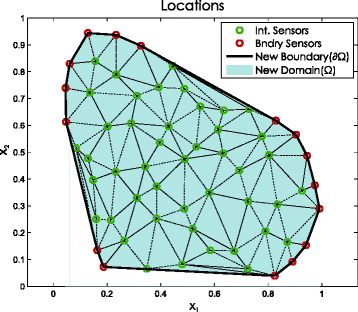

  

  A sensor network and its Delaunay triangulation. The monitored domain Ω partitioned into triangular meshes and the straight line segments making up the domain boundary ∂ Ω (black solid lines)

The assumption (a) above means that each sensor knows its position relative to other sensors in the network, this is important when recovering the location information of the unknown diffusion sources. Whilst the assumption (b), as will be seen in Section 5, is required in order for the nth sensor to be able to compute the weights with which to adjust its field measurements, before communicating them to neighboring sensors.

3 Gossip schemes for distributed average consensus

Gossiping [28, 29] is a distributed strategy for achieving consensus amongst agents in a network through a local exchange of data. Following the early works of [28] in the area, it has gained considerable interest for in-network processing in sensor networks as it mitigates the need for specialized routing protocols. In addition, gossip-based algorithms are robust to bottlenecks and link failures making it suitable for our distributed estimation problem. The results derived in this paper can be immediately extended to other gossiping schemes, such as those introduced in [30, 31]. An in-depth survey of gossiping algorithms in sensor networks is given in [29], and analysis of general averaging sum-weight-like algorithms in WSNs can be found in [32].

For the purpose of demonstration, in our simulation results, the archetypal pairwise randomized gossip algorithm [33] will be used. In this scheme, each node preserves an estimate of the sum and hence average of the node values. Let the value of node n after the ith pairwise gossip round be y _{n, i} , hence, y _{n, 0} is its initial value. In an iteration, a node n selected uniformly at random wakes up and contacts a randomly selected neighbor n ^′ within its connectivity radius, and they both update their estimates by setting $y_{n,\,i{+}1} = y_{n^{\prime },\,i{+}1} = \left (y_{n,\,i} {+} y_{n^{\prime },\,i}\right)/2$. Let y(i)=[y _{1, i} ,y _{2, i} ,…,y _{N, i} ]^T be the vector of the values of the N agents in the network at the ith gossip round, then this pairwise gossiping operation can be summarized in the following way

$$ \mathbf{y} (i+1) = \mathbf{P}(i) \mathbf{y}(i) $$

((4))

where P(i) are doubly stochastic matrices selected at random at the ith iteration. In the case of the pairwise gossip algorithm, P(i) has entries such that elements (n,n),(n,n ^′),(n ^′,n) and (n ^′,n ^′) are equal to 1/2 and is a diagonal identity elsewhere. Under this scheme, it can be shown that, if a network (of N nodes) is connected and each pair of nodes communicate often enough, the estimate at each node is guaranteed to converge to the global network average $\bar {y} = \frac {1}{N} \sum _{n=1}^{N} y_{n,\,0}$, i.e. ${\lim }_{i\rightarrow \infty } \mathbf {y}(i) = \mathbf {1}\bar {y}$. Performance guarantees and convergence results have also been studied (see [33] and the references therein).

The localized interactions in our field estimation setting will be based on the use of gossip algorithms for the distributed computation of a family of integrals whose final values can be used to reveal the unknown source parameters. In Section 5, we present our strategy for estimating these family of integrals and, hence, recover the unknown source parameters, through the use of gossip.

3.1 Quantized gossip

When the interactions between the agents are over a channel with finite capacity, the messages exchanged needs to be quantized. It is then natural to wonder if the values of the agents can still achieve consensus and converge to $\bar {Y}$ using the pairwise gossip scheme discussed previously. In what follows, we briefly investigate this question and briefly overview some proposed solutions in the literature. The inter-agent communication is through a channel employing a uniform quantizer with quantization step δ _Q . This communication can be modelled by introducing the quantization map $Q_{q}: \mathbb {R} \mapsto \mathcal {Q}$ such that

$$ Q_{q}(y) = k\delta_{Q}, \; \; \left(k - \frac{1}{2}\right)\delta_{Q} \leq y < \left(k + \frac{1}{2}\right)\delta_{Q}, $$

((5))

where $k \in \mathbb {Z}$ and $\mathcal {Q}$ is the set of permissible quantization levels, i.e. $\mathcal {Q} = \{ Q_{q}(y) : k \in \mathbb {Z}\}$.

3.1.1 Average consensus via naive quantized gossip

This is a straightforward extension of the standard gossip consensus scheme, whereby after each (pairwise) exchange of messages, the agents requantize their values and exchange this quantized value at the next iteration. It is summarized as follows,

$$ \mathbf{y}(i+1) = \mathbf{P}(i) Q_{q}(\mathbf{y}(i)), $$

((6))

where i denotes the ith iteration, Q _q denotes the mapping due to a uniform q-bit quantizer and P(i) is the transition matrix.

Under such a scheme, the agents in the network reach a consensus. However, convergence results are poor in the sense that the consensus value can be far away from the true average as is shown in Fig. 3 a. The poor convergence result observed is known to be due to the loss of symmetry between neighbors in the use of received information. Consequently, there has been considerable research efforts put towards devising average consensus strategies for networks with finite communication capacity, where it becomes impossible for sensors to exchange real numbers and hence arrive at the real-valued network average $\bar {Y}$.

Fig. 3

State evolution of quantized gossip schemes. Shows at each gossip iteration the state evolution of the agents in the network assuming a 5-bit uniform quantizer is used; the desired average is denoted by the dashed grey line. We use in a naive quantized gossip (NQG), b Kashyap’s quantized gossip (KQG) and c symmetric quantized gossip (SQG)

We consider in what follows some common quantized consensus strategies which are well suited to our field estimation task.

3.1.2 Kashyap’s quantized consensus gossip

In [34], Kashyap et al. propose a quantized consensus algorithm that aims to preserve the network average at every iteration. They prove that the collection of values at each agent in the network will converge to a quantized consensus distribution. Specifically, each node will converge to either $\bar {Y}$ or $\bar {Y} + 1$, where $\bar {Y} = \sum _{n=1}^{N} y_{n,0} \, \text {mod} \, N$, if the pair of communicating agents (n,n ^′) use an update such as

$$ \begin{aligned} y_{n,i+1} &= \left\lceil \frac{y_{n,i} + y_{n{'},i}}{2}\right\rceil, \\ y_{n{'},i+1} &= \left\lfloor \frac{y_{n,i} + y_{n',i}}{2}\right\rfloor, \end{aligned} $$

((7))

where $y_{n,i} \leq y_{n{^{\prime }},\,i}$, and ⌈·⌉, ⌊·⌋ is used to denote rounding up and down to the next quantizer level. We validate this approach through the simulation results shown in Fig. 3 b. We refer to [34] for a theoretical analysis of convergence.

3.1.3 Average consensus via symmetric quantized gossip

Frasca et al. [35] propose a scheme which aims to restore the symmetry lost by using an update scheme such as (6). This algorithm can be summarized as follows,

$$ \mathbf{y}(i+1) = \mathbf{y}(i) + \left(\mathbf{P}(i) - \mathbf{I}\right) Q_{q}(\mathbf{y}(i)) $$

((8))

where i denotes the ith iteration, Q _q is the mapping due to a uniform q-bit quantizer, P(i) is the diffusion (transition) matrix and I is the identity matrix.

Under such a scheme, the agents in the network achieve quantized consensus in the sense that the value at each node is at most one quantizer level away from the true average. Specifically, as well as the total sum of the states being preserved, the states of the agents in the network converge but to different values which are close to the true average, and in fact only differ from this true average by at most one bin. This can be seen in Fig. 3 c which shows the state evolution of the agents in the network assuming a 5-bit (32-level) uniform quantizer.

4 Centralized recovery of multiple sources

In what follows, we provide an overview for the centralized recovery of diffusion fields as proposed in [36], wherein we demonstrate through the use of Green’s second theorem that given access to some generalized measurements of the form

$$ \mathcal{R}(k)\! = \! \left\langle \Psi_{k}(\mathbf{x}) \Gamma(t), f \right\rangle \! = \! \int_{\Omega} \! \int_{t} \! \Psi_{k}(\mathbf{x}) \Gamma(t) f(\mathbf{x},t) \mathrm{d}t\mathrm{d}V, $$

((9))

for k=0,1,…,K, it is possible to uniquely determine the unknown source parameters in f(x,t), provided Ψ _k (x) and Γ(t) are spatial and temporal sensing functions, respectively, chosen to satisfy certain conditions. In (9), V is the variable of integration performed over a surface Ω. We will see that if Ψ _k (x) and Γ(t) are properly chosen, the integrals in (9) reduce to a power-sum series which can be efficiently solved using Prony’s method to recover the unknown source parameters.

4.1 Closed-form inversion

Let us commence by relating the field u(x,t) diffusing in Ω to the unknown sources inducing the field, through the use of Green’s second theorem. Denote by Ψ _k an arbitrary twice differentiable function in Ω, then Green’s second identity relates the boundary and the surface integrals over the bounded region as follows,

$$ \oint_{\partial \Omega}\!\! \left({\Psi_{k}\nabla u \,-\, u\nabla\Psi_{k}}\right)\cdot \hat{\mathbf{n}}_{\partial \Omega} \mathrm{d}S\! =\!\!\int_{\Omega} \!\! \left({\Psi_{k}\nabla^{2} u \,-\, u\nabla^{2}\Psi_{k}}\right) \mathrm{d}V, $$

((10))

where $\hat {\mathbf {n}}_{\partial \Omega }$ is the outward pointing unit normal vector to the boundary ∂ Ω of Ω, and S denotes the variable of integration along the boundary ∂ Ω of Ω.

Furthermore, if Ψ _k is chosen to satisfy

$$ \frac{\partial \Psi_{k}}{\partial t} + \mu \nabla^{2} \Psi_{k} = 0, $$

((11))

then by substituting (1) and $\nabla ^{2} \Psi _{k} = - \frac {1}{\mu } \frac {\partial \Psi _{k}}{\partial t}$ into (10), we obtain

$$ \int_{\Omega} \! { \frac{\partial}{\partial t} (\!u\Psi_{k}\!)} \mathrm{d}V \,-\,{\mu}\!\oint_{\partial \Omega}\!\!\left({\Psi_{k}\nabla u - u\nabla\Psi_{k}}\!\right)\!\cdot\! \hat{\mathbf{n}}_{\partial \Omega} \mathrm{d}S\! =\!\! \int_{\!\Omega}\!\! {\Psi_{k} \,f} \mathrm{d}V. $$

((12))

This is the basis of the reciprocity gap (RG) method [37] used in non-destructive testing of solids [37, 38]. Essentially, if u(x,t) is known and since we choose and therefore also know Ψ _k (x), the left hand side (lhs) of (12) can be computed. We show in what follows how it is possible to recover f(x,t) algebraically from this, under certain conditions.

Remark 1.

Equation (11) is the so-called adjoint of the diffusion equation, and in this work, we will refer to any family of functions that satisfy this equation as a spatial sensing function.

Firstly, we extend the reciprocity gap method by multiplying both sides of the so-called reciprocity gap functional, (12), by a time-varying sensing function Γ(t) and then integrating the resulting expression over t∈ [ 0,T], to obtain

$$ {\fontsize{9.2}{6}\begin{aligned} &\underbrace{\int_{t=0}^{T} \Gamma(t) \left(\!\int_{\Omega} \! { \frac{\partial}{\partial t} (u\Psi_{k}\!)} \mathrm{d}V \,-\,{\mu}\! \oint_{\partial \Omega}\!\!\left({\Psi_{k}\nabla u - u\nabla\Psi_{k}}\!\right)\!\cdot\! \hat{\mathbf{n}}_{\partial \Omega} \mathrm{d}S \!\right) \mathrm{d}t\!}_{\stackrel{\text{\tiny{def}}}{=} \mathcal{R}(k)}\\ &\quad= \int_{t=0}^{T} \Gamma(t) \int_{\!\Omega}\!\! {\Psi_{k} f} \mathrm{d}V\mathrm{d}t. \end{aligned}} $$

((13))

Notice that (13) now depends only on k and coincides with (9) if we denote its lhs with $\mathcal {R}(k)$. Specifically,

$$ \mathcal{R}(k)\! = \! \left\langle \Psi_{k}(\mathbf{x}) \Gamma(t), f \right\rangle \! = \! \int_{\Omega} \! \int_{t} \! \Psi_{k}(\mathbf{x}) \Gamma(t) f(\mathbf{x},t) \mathrm{d}t\mathrm{d}V. $$

((14))

Moreover, for a time-independent choice of Ψ _k (x), we have that

$$ {{\begin{aligned} \mathcal{R}(k) = \! \int_{\Omega} \! (\Psi_{k} \dot{U})(\mathbf{x}, T) \mathrm{d}V \! - {\mu} \!\oint_{\partial \Omega} \! \left({\Psi_{k}\nabla U - U\nabla\Psi_{k}}\right)\cdot \hat{\mathbf{n}}_{\partial \Omega} \mathrm{d}S, \end{aligned}}} $$

((15))

where

$$\begin{array}{*{20}l} U(\mathbf{x},T) &= {\int_{0}^{T}} \Gamma(t) u(\mathbf{x},t) \mathrm{d}t \; \text{and,} \end{array} $$

((16a))

$$\begin{array}{*{20}l} \dot{U}(\mathbf{x},T) &= \Gamma(T) u(\mathbf{x},T) - {\int_{0}^{T}} \frac{\partial \Gamma}{\partial t} u (\mathbf{x},t) \mathrm{d}t. \end{array} $$

((16b))

Hence, $\mathcal {R}(k)$ can be computed exactly if u(x,t), Ψ _k (x) and Γ(t) are known over Ω×[ 0,T]. We now demonstrate how to choose the spatial and temporal sensing functions so that given $\mathcal {R}(k)$, the unknown parameters of f(x,t) can be retrieved. We first observe the following fact:

Lemma 1.

$\Psi _{k}(\mathbf {x}) = e^{-k(x_{1}\phantom {\dot {i}\!} + \mathrm {j} x_{2})}$ is a valid spatial sensing function.

Proof.

A valid spatial sensing function in our context must satisfy (11) in order to obtain (12) from (10). Notice that $\Psi _{k}(\mathbf {x})= e^{-k(x_{1}\phantom {\dot {i}\!} + \mathrm {j} x_{2})}$ is time independent; and also analytic (i.e. ∇² Ψ _k =0), which follows by summing its second derivatives with respect to x ₁ and x ₂. Combining these two properties allows us to conclude that $\frac {\partial \Psi _{k}}{\partial t} + \mu \nabla ^{2} \Psi _{k} = 0$.

Therefore, (15) is satisfied when we choose Γ(t) to be the time-varying function Γ(t)=e ^−jt/T, and $\Psi _{k}(\mathbf {x}) = e^{-k(x_{1}\phantom {\dot {i}\!} + \mathrm {j} x_{2})}$ which by Lemma 1 is a valid sensing function. Furthermore, for the source parameterization (3), the right hand side of (14) becomes, $\mathcal {R}(k) = \sum _{m=1}^{M} c_{m} \Gamma (\tau _{m}) \Psi _{k}(\boldsymbol {\xi }_{m})$, which results in the following power-sum series:

$$ \mathcal{R}(k) = \sum_{m=1}^{M} c_{m} e^{-\mathrm{j}\tau_{m}/T} e^{-k \left(\xi_{1,m} + \mathrm{j}\xi_{2,m}\right)}, \; \; k = 0,1,\ldots,K, $$

((17))

when replacing Γ(t) with e ^−jt/T and Ψ _k (x) with $e^{-k(x_{1}\phantom {\dot {i}\!} + \mathrm {j} x_{2})}$. Equation (17) is a Prony system frequently encountered in spectral estimation [39] and within the finite rate of innovation framework [40] and can be solved to obtain all M pairs $\left \{c_{m} e^{-\mathrm {j} \tau _{m}/T}, \xi _{1,m} + \text {j} \xi _{2,m}\right \}^{M}_{m=1}$, and therefore, $\left \{c_{m}, \tau _{m}, \boldsymbol {\xi }_{m}\right \}_{m=1}^{M}$ if K≥2M−1. A brief overview of the essential elements of Prony’s method is given in Appendix A; for a more in-depth treatment, we refer to [40, 41].

In practice, the sequence $\{\mathcal {R}(k)\}_{k=0}^{K}$ cannot be computed exactly using (15) since we do not have access to the entire field u(x,t) but only to sensor measurements $\{\varphi _{n}(t_{l}): l=0,1,\ldots,L \}_{n=1}^{N}$. A way to compute good approximations of (15) using standard quadrature techniques is discussed in [36]. When using these quadrature techniques to obtain an approximation of the generalized measurements $\{ \mathcal {R}(k)\}_{k}$, the performance of the centralized algorithm is near-optimal, in that it comes very close to achieving the Cramer-Rao bound (CRB) as shown in Fig. 10.

In the next section, we present a novel consensus-type method for the distributed estimation of $\{\mathcal {R}(k)\}_{k}$ that is able to achieve the same estimation performance as the centralized estimation algorithm, using only local exchanges of the sensor measurements.

5 Towards a distributed source recovery: physics-based consensus

As highlighted in Section 2, we assume that the sensors know the topology of the network and that each sensor performs the Delaunay triangulation as shown in Fig. 2.

5.1 Consensus-based estimation over sensor networks

With the assumptions above, we can now derive the consensus-based diffusion source estimation scheme as follows.

Firstly, consider the surface integral contribution in (15), and the triangulation of Fig. 2, if the bounded domain Ω is partitioned into non-overlapping triangular subdivisions $\left \{\!\Delta _{j}\right \}_{j=1}^{J}$ such that $\bigcup _{i=1}^{I} \Delta _{i} = \Omega$ and $\Delta _{i} \bigcap \Delta _{j} = \emptyset$ for i≠j, then this integral can be approximated by the sum [42]:

$$ \int_{\Omega} \!\! \left(\Psi_{k} \dot{U}\right)(\mathbf{x}, T) \, \mathrm{d}V \!\approx\!\! \frac{1}{3}\! \sum_{j=1}^{J} \sum_{j'=1}^{3}\! \Psi_{k}\left(\mathbf{v}_{j,j'}\!\right) \dot{\Phi}_{j,j'}(t_{L}) {|\Delta_{j}|}, $$

((18))

where $\mathbf {v}_{j,\,j^{\prime }}$ is the j ^′th vertex of triangle j and $\dot {\Phi }_{j,\,j'}(t_{L}) = \dot {U}(\mathbf {v}_{j,\,j'},t_{L})$ is the measurement of the sensor situated at this vertex at time t=t _L =T. Moreover, the double sum, in (18), can be re-written in the following way:

$$ {\fontsize{9.2}{6}\begin{aligned} \int_{\Omega} \! \left(\Psi_{k} \dot{U}\right)(\mathbf{x}, T) \, \mathrm{d}V & \approx \frac{1}{3}\! \sum_{j=1}^{J} \sum_{j'=1}^{3}\! \Psi_{k}\left(\mathbf{v}_{j,j'}\!\right) \dot{\Phi}_{j,j'}(t_{L}) |\!\Delta_{j}\!|\\ &= \frac{1}{3} \sum_{j=1}^{J} \! |\!\Delta_{j}| \!\left(\Psi_{k}\left(\mathbf{v}_{j,\,1}\!\right)\dot{\Phi}_{j,1}(t_{L})\right.\\ &\left. \quad+ \Psi_{k}\left(\mathbf{v}_{j,\,2}\!\right)\dot{\Phi}_{j,\,2}(t_{L}) \,+\, \Psi_{k}\left(\mathbf{v}_{j,\,3}\!\right)\!\dot{\Phi}_{j,\,3}(t_{L}) \right) \\ &= \sum_{n=1}^{N} \underbrace{\left(\frac{1}{3}\Psi_{k}(\mathbf{x}_{n}) \sum_{j=1}^{J_{n}} |\!\Delta_{n,j}| \right)}_{:=A_{n}(k)} \dot{\Phi}_{n}(t_{L}) \end{aligned}} $$

((19))

where Δ _{n, j} and | Δ _{n, j} | are used to denote the jth triangle and its area, respectively, for which node n is a vertex. The last equality follows by noticing that $\dot {\Phi }_{j,\,j'}(t_{L})$ is always weighted by the product of the area of triangle j and $1/3\Psi _{k}(\mathbf {v}_{j,\,j^{\prime }})$. Hence, denoting the set of all triangles that share a common vertex n located at x _n by $\mathcal {T}_{n} = \{\Delta _{n,1},\Delta _{n,2}, \ldots, \Delta _{n,J_{n}}\}$, the measurement $\dot {\Phi }_{n}(t_{L})$ is always weighted by the sum of the areas of its corresponding triangles and 1/3Ψ _k (x _n ). We denote this weight that directly depends on the sensing function and Delaunay triangulation (equivalently, the topology of the network) by A _n (k).

For the boundary integral, the time-integrated field U(x) and its spatial derivative $\nabla U(\!\mathbf {x}\!) {=} \left [ \frac {\partial U}{\partial x_{1}}, \frac {\partial U}{\partial x_{2}} \right ]^{\mathsf {T}}\,=\,\left [ U_{x_{1}}, U_{x_{2}}\right ]^{\mathsf {T}}$ are required. Let $\mathcal {S}_{\partial \Omega } = \{1, \ldots, n, \ldots, I\}$ denote the cyclically ordered set of the boundary sensors; these coincide with the vertices of the convex hull. Furthermore, assume the elements of $\mathcal {S}_{\partial \Omega }$ are in counterclockwise order, then, $\hat {\mathbf {n}}_{\partial \Omega } \mathrm {d}S \approx \left [ x_{2,n} {-} x_{2,n{-}1}, x_{1,n{-}1} {-} x_{1,n}\right ]^{\mathsf {T}}$. Hence, the boundary integral can be approximated as follows,

$$ {}\begin{aligned} &\oint_{\partial \Omega} \left({\Psi_{k}\nabla U - U\nabla\Psi_{k}}\right)\cdot \hat{\mathbf{n}}_{\partial \Omega} \, \mathrm{d}S\\ &\approx \sum_{n=1}^{I} \Psi_{k}(\mathbf{x}_{n}) \left[ \left(U_{x_{1}}(\mathbf{x}_{n}) + k U(\mathbf{x}_{n})\right)\left(x_{2,n} - x_{2,n-1}\right) \right.\\ & \quad + \left. \left(U_{x_{2}}(\mathbf{x}_{n}) + \mathrm{j} k U(\mathbf{x}_{n})\right)\left(x_{1,n-1} - x_{1,n}\right) \right]\\ & =\sum_{n=1}^{I}\!\!\Psi_{k}(\!\mathbf{x}_{n}\!)\!\left\{\! \left(\!x_{2,n}\! -\! x_{2,n\,-\,1}\!\right)U_{x_{1}}(\!\mathbf{x}_{n}\!) \,+\, \left(\!x_{1,n\,-\,1}\! -\! x_{1,n}\!\right) U_{x_{2}}(\!\mathbf{x}_{n}\!) \right.\\ & \quad + \left. U(\mathbf{x}_{n}) \left[ \left(x_{2,n} - x_{2,n-1}\right) + \mathrm{j} \left(x_{1,n-1} - x_{1,n}\right) \right] \right\}. \end{aligned} $$

((20))

The first term in (20) depends on U(x _n ) and its spatial derivative which must be approximated from spatiotemporal samples of u(x,t). Note that U(x _n ) can be obtained by sensor n independently using trapezium rule. However, ∇U(x _n ) can only be estimated reliably using neighboring sensor measurements by a polynomial fitting approach. Specifically, we find the regression function U(x _n )=α _n x _1,n +β _n x _2,n +γ _n by estimating (α _n ,β _n ,γ _n ) for each boundary sensor n=1,…,I using measurements of the nearest neighbors to the point x _n .

Let the nth sensor located at x _n , with measurement U(x _n ) have the two closest sensors x n′ and x n″ with corresponding measurements U(x n′) and U(x n″). With these, we can estimate the parameters (α _n ,β _n ,γ _n ) by solving the linear system:

$$\begin{array}{*{20}l} \left[\begin{array}{c} U(\mathbf{x}^{\prime\prime}_{n}) \\ U(\mathbf{x}_{n}) \\ U(\mathbf{x}^{\prime}_{n})\end{array}\right] &= \left[\begin{array}{ccc} x^{\prime\prime}_{1,n} & x^{\prime\prime}_{2,n} & 1 \\ x_{1,n} & x_{2,n} & 1 \\ x^{\prime}_{1,n}& x^{\prime}_{2,n}& 1 \end{array}\right] \left[\begin{array}{c} \alpha_{n} \\ \beta_{n} \\ \gamma_{n} \end{array}\right], \end{array} $$

((21))

$$\begin{array}{*{20}l} \mathbf{u}_{n} &= \mathbf{X}_{n} \mathbf{d}_{n}. \end{array} $$

((22))

The system admits a unique solution, if x n″,x _n and x n′ are not collinear. Therefore, the local spatial derivative ∇U(x _n ) can be retrieved directly from the solution to this system by noticing that the polynomial p(x)=α x ₁+β x ₂+γ has ∇p(x)=〈α,β〉. Hence, $\nabla U(\mathbf {x}_{n}) = \left [ U_{x_{1}}(\mathbf {x}_{n}), U_{x_{2}}(\mathbf {x}_{n}) \right ]^{\mathsf {T}} \approx \left [ \alpha _{n}, \beta _{n} \right ]^{\mathsf {T}}$, where

$$\begin{aligned} \alpha_{n} &{=}\frac{\left(x_{2,n}\! {-} x^{\prime}_{2,n}\right)U(\mathbf{x}^{\prime\prime}_{n}) {+} \left(x^{\prime}_{2,n} \!{-} x^{\prime\prime}_{2,n}\right)U(\mathbf{x}_{n}) {+} \left(x^{\prime\prime}_{2,n} \!{-} x_{2,n}\right)U(\mathbf{x}^{\prime}_{n})}{\det(\mathbf{X}_{n})},\\ \beta_{n} &{=} \frac{\left(x^{\prime}_{1,n}\! {-} x_{1,n}\right)U(\mathbf{x}^{\prime\prime}_{n}) {+} \left(x^{\prime\prime}_{1,n}{-}x^{\prime}_{1,n}\right)U(\mathbf{x}_{n}) {+}\left(x_{1,n}{-} x^{\prime\prime}_{1,n}\right)U(\mathbf{x}^{\prime}_{n})}{\det(\mathbf{X}_{n})}\!. \end{aligned} $$

Then, substituting these back into (20) gives

$$ \begin{aligned} &\oint_{\partial \Omega} \left({\Psi_{k}\nabla U - U\nabla\Psi_{k}}\right)\cdot \hat{\mathbf{n}}_{\partial \Omega} \, \mathrm{d}S \\ &\quad \approx \sum_{n=1}^{I} b^{\prime\prime}_{n}(k) U(\mathbf{x}^{\prime\prime}_{n}) + b_{n}(k) U(\mathbf{x}_{n}) + b^{\prime}_{n}(k) U(\mathbf{x}^{\prime}_{n}), \end{aligned} \vspace*{-2mm} $$

((23))

where

$$\begin{array}{*{20}l} b^{\prime\prime}_{n}(k){=}\frac{\Psi_{k}(\mathbf{x}_{n})}{\det(\mathbf{X}_{n})} \left[\! \begin{array}{c} x_{1,n-1} \,-\, x_{1,n}\\ x_{2,n}\! -\! x_{2,n-1}\end{array}\!\right]^{\mathsf{T}} \!\!\left[\!\begin{array}{c} x^{\prime}_{1,n}\! -\! x_{1,n}\\ x_{2,n}\! -\! x^{\prime}_{2,n} \end{array}\!\right], \end{array} $$

((24a))

$$\begin{array}{*{20}l} b_{n}(k) &{=}\frac{\Psi_{k}(\mathbf{x}_{n})}{\det(\mathbf{X}_{n})} \left[\! \begin{array}{c} x_{1,n-1} \,-\, x_{1,n}\\ x_{2,n}\! -\! x_{2,n-1}\end{array}\!\right]^{\mathsf{T}} \!\!\left[\!\begin{array}{c} x^{\prime\prime}_{1,n} \,-\, x^{\prime}_{1,n}\\ x^{\prime}_{2,n}\! -\! x^{\prime\prime}_{2,n} \end{array}\!\right] \\ &\quad{+} k \Psi_{k}(\mathbf{x}_{n})\left[\!\left(x_{2,n} {-} x_{2,n-1}\right){+} \mathrm{j} \left(x_{1,n-1}{-} x_{1,n}\right)\!\right], \end{array} $$

((24b))

$$\begin{array}{*{20}l} b'_{n}(k){=}\frac{\Psi_{k}(\mathbf{x}_{n})}{\det(\mathbf{X}_{n})}\left[\!\begin{array}{c} x_{1,n-1} \,-\, x_{1,n}\\ x_{2,n} \!- \!x_{2,n-1} \end{array}\!\right]^{\mathsf{T}} \!\!\left[\! \begin{array}{c} x_{1,n}\! -\! x^{\prime\prime}_{1,n}\\ x^{\prime\prime}_{2,n} \,-\, x_{2,n}\end{array}\!\right]. \end{array} $$

((24c))

The terms b n″(k),b _n (k) and $b^{\prime }_{n}(k)$ in (24a) are dependent only on the topology of the network (specifically the locations of the sensors) and our choice of sensing function Ψ _k (x). Indeed given the assumptions detailed in Section 2, these weights can be precomputed for every sensor in the network, such that

$$ \oint_{\partial \Omega} \left({\Psi_{k}\nabla U - U\nabla\Psi_{k}}\right)\cdot \hat{\mathbf{n}}_{\partial \Omega} \, \mathrm{d}S \approx \sum_{n \in \mathcal{S}} B_{n}(k) U(\mathbf{x}_{n}), $$

((25))

where B _n (k) is non-zero if n is a boundary sensor, i.e. $n \in \mathcal {S}_{\partial \Omega }$, or if it is one of the two nearest sensors to a boundary sensor, $n \in \mathcal {N}_{\partial \Omega }$. Otherwise, B _n (k) is zero. Finally, we can combine (19) and (25), to obtain the estimates for $\mathcal {R}(k)$:

$$\begin{array}{*{20}l} \mathcal{R}(k) &\approx \sum_{n \in \mathcal{S}} A_{n}(k) \dot{\Phi}_{n}(t_{L}) - \mu B_{n}(k) \Phi_{n}(t_{L}) \end{array} $$

((26))

$$\begin{array}{*{20}l} &= \frac{1}{N}\sum_{n \in \mathcal{S}} y_{n}(k). \end{array} $$

((27))

where

$$ y_{n}(k) = N \left(A_{n}(k) \dot{\Phi}_{n}(t_{L}) - \mu B_{n}(k) \Phi_{n}(t_{L}) \right). $$

((28))

Upon deployment of the sensors, each sensor can precompute its unique weights {A _n (k)} _k and {B _n (k)} _k for k=0,…,K. This is possible as a result of the assumptions (a) and (b) stated in Section 2. After which they can start to monitor the region of interest Ω, by sensing the field locally. To initiate the estimation process, the sensor n exchanges its modified measurements {y _n (k)} _k with a randomly chosen neighbor. This begins the gossip round, as detailed in Section 3; it continues until convergence to $\{\mathcal {R}(k)\}_{k}$. All sensors in the network can now independently apply Prony’s method to its current estimate of $\{\mathcal {R}(k)\}_{k}$ in order to recover all M triples {c _m ,τ _m ,ξ _m } as described in Section 4.1. Consequently, we can now state the following proposition:

Proposition 1.

By exchanging the properly weighted sum of sensor measurements, $y_{n}(k) {=} N\left [A_{n}(k) \dot {\Phi }_{n}(t_{L}) -\right. \left.\mu B_{n}(k) \Phi _{n}(t_{L})\right ]$, it is possible for each sensor n to converge to the same generalized measurements $\{ \mathcal {R}(k)\}_{k}$ as the centralized algorithm and hence recover the unknown diffusion source parameters with the same estimation performance. Here, A _n (k) and B _n (k) are dependent on Ψ _k and the topology of the network, whilst Φ _n (t _L ) and $\dot {\Phi }_{n}(t_{L})$ are approximations of the time integrals ( 16a ) and ( 16b ), respectively, obtained by sensor n at location x=x _n , with T=t _L .

5.2 Noise robust consensus-based estimation

Proposition 1 presents a gossiping strategy for noiseless measurements. In a noisy scenario, while the basic strategy stays the same, some further processing is required to improve noise resilience.

In the presence of measurement noise, the sensors in the network obtain noisy spatiotemporal samples of the field:

$$ \varphi_{n}^{\epsilon}(t_{l}) = \varphi_{n}(t_{l}) + {\epsilon}_{n,l}, $$

((29))

where we assume that {ε _n,l } are independent and identically distributed such that ${\epsilon }_{n,l} \sim \mathcal {N}\left (0,\sigma ^{2}\right)$ for n∈{1,2,…,N} and l∈{0,1,…,L}.

In Proposition 1, the sensors exchange their local measures {y _n (k)} _k with neighboring nodes in order to obtain a consensus on the desired generalized measurements $\{ \mathcal {R}(k) \}_{k}$. Recall that for each k, y _n (k)=N(A _n (k)Φ̇ _n (t _L )−μ B _n (k)Φ _n (t _L )), this is simply a weighted sum of the temporal field measurements taken by sensor n; thus, we can write $y_{n}(k) = \sum _{l=0}^{L} w_{n,l}(k)\varphi _{n}(t_{l})$, with $w_{n,l}(k) \in \mathbb {C}$ since $A_{n}(k), B_{n}(k) \in \mathbb {C}$. Therefore, in the noisy setting, the sensors exchange

$$\begin{array}{*{20}l} y_{n}^{\epsilon}(k) &= \sum_{l=0}^{L} w_{n,l}(k) \varphi_{n}^{\epsilon}(t_{l}) = \sum_{l=0}^{L} w_{n,l}(k) \left(\varphi_{n}(t_{l}) + {\epsilon}_{n,l} \right) \\ &= y_{n}(k) + \sum_{l=0}^{L} w_{n,l}(k) {\epsilon}_{n,l}. \end{array} $$

((30))

We now consider the consensus value; upon convergence, each sensor in the network holds: $\left \{ \mathcal {R}^{\epsilon }(k) = \frac {1}{N} \sum _{n=1}^{N} y_{n}^{\epsilon }(k) \right \}_{k{=}0}^{K}$ from which they construct the Toeplitz matrix, i.e. $\text {Toep}\left (\left \{ \mathcal {R}^{\epsilon }(k) \right \}_{k{=}0}^{K}\right)$, in order to apply Prony’s method. In the noisy scenario, they will instead construct (see also Appendix A),

$$ {{ \begin{aligned} {} \text{Toep}\left(\{ \mathcal{R}^{\epsilon}(k) \}_{k}\right) &\,=\, \text{Toep}\left(\left\{ \frac{1}{N} \sum_{n=1}^{N} y_{n}^{\epsilon}(k) \right\}_{k}\right) \\ &\,=\, \text{Toep}\left(\{ \mathcal{R}(k) \}_{k}\right) \,+\, \text{Toep}\left(\left\{ \frac{1}{N} \sum_{n=1}^{N} \sum_{l=0}^{L} w_{n,l}(k) {\epsilon}_{n,l} \right\}_{k}\right) \\ &\,=\, \text{Toep}\left(\left\{ \mathcal{R}(k) \right\}_{k}\right) + \text{Toep}\left(\left\{ \epsilon(k) \right\}_{k}\right) \\ &\,=\, \text{Toep}\left(\left\{\mathcal{R}(k) \right\}_{k}\right) + \mathbf{T}_{\epsilon}. \end{aligned}}} $$

((31))

It is clear that, the noise term in $\text {Toep}\left (\left \{ \mathcal {R}^{\epsilon }(k) \right \}_{k{=}0}^{K}\right)$, given noisy spatiotemporal sensor measurements becomes colored due to the weighted sum. However, Prony’s method and its variations implicitly assume that the noise in the terms $\{\mathcal {R}^{\epsilon }(k) \}_{k}$ are i.i.d, hence it must be pre-whitened before estimating the unknown source parameters from it. To this end, each sensor can design and apply (by post-multiplying the Toeplitz matrix $\text {Toep}\left (\{ \mathcal {R}^{\epsilon }(k) \}_{k}\right)$ with) the pre-whitening filter F given by

$$ \mathbf{F} = \mathbf{C}_{\epsilon}^{\frac{\dagger}{2}} $$

((32))

where $(\cdot)^{\frac {\dagger }{2}}$ is the square root of the Moore-Penrose pseudoinverse, and

$$ \mathbf{C}_{\epsilon} = \text{Cov}\{ \mathbf{T}_{\epsilon} \} = \mathbb{E}\left\{ \mathbf{T}_{\epsilon} \mathbf{T}_{\epsilon}^{\mathsf{H}} \right\}, $$

((33))

before applying Prony’s method.

Notice that the covariance matrix, C _ε , depends directly on the variance of the sensor noise and on the weights {w _{n, l} (k)} _n,l (hence, the network topology) for any k∈{0,1,…,K}. In what follows, we derive explicitly an expression for C _ε .

For ease of exposition, we define the matrix of coefficients $\mathbf {W} (k) \in \mathbb {C}^{N\times (L+1)}$, such that its entries are given by [W(k)] _{n, l+1}=w _n,l (k). Then, we define the vector of coefficients $\mathbf {w}(k) = \text {vec}\left (\mathbf {W}(k)\right)$ to be the vectorization of W(k)—i.e. $\mathbf {w}(k) \in \mathbb {C}^{N(L+1)}$ is formed by stacking the columns of the matrix W(k) into a single column vector. Similarly, let $\boldsymbol {\epsilon } \in \mathbb {R}^{N(L+1)}$ be the vector formed from the i.i.d noise sequence {ε _n,l } _{n, l} in the same way. Thus, $\epsilon (k) = \frac {1}{N} \sum _{n=1}^{N} \sum _{l=0}^{L} w_{n,\,l}(k) \epsilon _{n,l} = \frac 1N \mathbf {w}^{\mathsf {T}}(k) \boldsymbol {\epsilon }$. From this, if $\mathbf {T}_{\epsilon } \in \mathbb {R}^{N_{1} \times N_{2}}$ for instance, i.e.

$$\left[\begin{array}{cccc} \epsilon(N_{2}{-}1) & \epsilon(N_{1} {-} 2) & \cdots & \epsilon(0) \\ \epsilon(N_{2}) & \epsilon(N_{2}{-}1) & \cdots & \epsilon(1) \\ \vdots & \vdots & \ddots & \vdots \\ \epsilon(N_{1} {+}N_{2}{-}2) & \epsilon(N_{1} {+}N_{2}{-}3) & \cdots & \epsilon(N_{1}{-}1) \\ \end{array}\right], $$

we may write

$${ \fontsize{5.9}{15}\selectfont{\begin{aligned} \mathbf{C}_{\epsilon} &= \mathbb{E}\left\{ \mathbf{T}_{\epsilon} \mathbf{T}_{\epsilon}^{\mathsf{\!H}} \right\} \\ &= \mathbb{E} \left\{\!\! \left[\!\! \begin{array}{cccc} \sum\limits_{i=0}^{N_{2} {-} 1}\epsilon(i)\epsilon^{\mathsf{\!H}}\!(i) & \sum\limits_{i=0}^{N_{2}{-}1} \epsilon(i)\epsilon^{\mathsf{\!H}}\!(i {+} 1) & \cdots & \sum\limits_{i=0}^{N_{2}{-}1} \epsilon(i)\epsilon^{\!\mathsf{H}}\!(i {+}N_{1} {-} 1) \\ \sum\limits_{i=0}^{N_{2}{-}1} \epsilon(i{+}1)\epsilon^{\!\mathsf{H}}\!(i) & \sum\limits_{i=0}^{N_{2}{-}1} \epsilon(i {+}1)\epsilon^{\!\mathsf{H}}\!(i {+}1) & \cdots & \sum\limits_{i=0}^{N_{2}{-}1} \epsilon(i {+}1)\epsilon^{\!\mathsf{H}}\!(i {+}N_{1} {-}1) \\ \vdots & \vdots & \ddots & \vdots \\ \!\sum\limits_{i=0}^{N_{2}{-}1} \epsilon(i{+}N_{1}{-}1)\epsilon^{\!\mathsf{H}}\!(i) & \sum\limits_{i=0}^{N_{2}{-}1} \epsilon(i{+}N_{1}{-}1)\epsilon^{\mathsf{H}}\!(i {+}1) & \cdots & \sum\limits_{i=0}^{N_{2}{-}1} \epsilon(i{+}N_{1}{-}1)\epsilon^{\!\mathsf{H}}\!(i {+}N_{1} {-}1) \\ \end{array} \!\!\right] \!\!\right\}. \end{aligned}}} $$

Taking the expectation operator inside the matrix and noting that

$$\begin{array}{*{20}l} \mathbb{E}\left\{ \sum_{i=0}^{N_{2}-1} \epsilon(i{+}j) \epsilon^{\!\mathsf{H}}(i) \right\} &= \mathbb{E}\left\{ \sum_{i=0}^{N_{2}-1} \epsilon(i) \epsilon^{\mathsf{H}}(i{+}j) \right\} \\ &= \frac{1}{N^{2}} \sum_{i=0}^{N_{2}-1} \mathbb{E}\left\{\mathbf{w}^{\!\mathsf{T}}(i) \boldsymbol{\epsilon} \boldsymbol{\epsilon}^{\mathsf{H}} \mathbf{w}^{*}\!(i{+}j) \right\} \\ &= \frac{1}{N^{2}} \sum_{i=0}^{N_{2}{-}1} \mathbf{w}^{\!\mathsf{T}}(i) \left(\sigma^{2} \mathbf{I}\right) \mathbf{w}^{*}\!(i{+}j) &\\ &= \frac{\sigma^{2}}{N^{2}} \sum_{i=0}^{N_{2}{-}1} \mathbf{w}^{\!\mathsf{T}}(i) \mathbf{w}^{*}\!(i{+}j), \end{array} $$

allows us to write the covariance matrix (33) in the form

$$ {\fontsize{6.2}{9.6}\selectfont{\begin{aligned} {}\mathbf{C}_{\epsilon} {=} \frac{\sigma^{2}}{N^{2}}\!\! \left[\!\! \begin{array}{cccc} \sum\limits_{i=0}^{N_{2} {-} 1} \!\! \|\mathbf{w}(i)\|^{\!2} & \sum\limits_{i=0}^{N_{2}{-}1} \!\! \mathbf{w}^{\!\mathsf{T}}\!(i)\mathbf{w}^{*}\!(i {+} 1) & \cdots & \sum\limits_{i=0}^{N_{2}{-}1} \!\! \mathbf{w}^{\!\mathsf{T}}\!(i)\mathbf{w}^{*}\!(i {+}N_{1} {-} 1) \\ \sum\limits_{i=0}^{N_{2}{-}1} \!\! \mathbf{w}^{\!\mathsf{T}}\!\!(i{+}1)\mathbf{w}^{*}\!(i) & \sum\limits_{i=0}^{N_{2}{-}1} \!\! \|\mathbf{w}(i {+}1)\|^{\!2} & \cdots & \sum\limits_{i=0}^{N_{2}{-}1} \!\! \mathbf{w}^{\!\mathsf{T}}\!(i {+}1) \mathbf{w}^{*}\!(i {+}N_{1}{-}1) \\ \vdots & \vdots & \ddots & \vdots \\ \!\sum\limits_{i=0}^{N_{2}{-}1} \!\! \mathbf{w}^{\!\mathsf{T}}\!(i{+}N_{1}{-}1)\mathbf{w}^{*}\!(i) & \sum\limits_{i=0}^{N_{2}{-}1} \!\! \mathbf{w}^{\!\mathsf{T}}\!(i{+}N_{1}{-}1)\mathbf{w}^{*}\!(i {+}1) & \cdots & \sum\limits_{i=0}^{N_{2}{-}1} \!\! \|\mathbf{w}(i {+}N_{1} {-}1)\|^{\!2}\\ \end{array} \!\!\!\right]. \end{aligned}}} $$

((34))

To further improve the noise robustness of our source estimation approach, we adapt the sequential local line search technique introduced [36]. This modification is based on searching for a time interval over where only a single diffusion source is active. When such an interval is found, the active source parameters are estimated and its contribution to the spatiotemporal field measurements is removed before the next source can be estimated. In summary, this is achieved by considering an initial time interval [ 0,T] and doing the following:

• 1. Assume there are M ^′≥2 unknown sources. Approximate $\{\mathcal {R}^{\epsilon }(k)\}_{k=0}^{2M' - 1}$ using the gossiping approach as described in Section 5.1.

• 2. Estimate the M ^′ source intensities $\left \{\sigma '_{m'}\right \}_{m'=1}^{M'}$ and locations $\left \{\boldsymbol {\xi }'_{m'}\right \}_{m'=1}^{M'}$ using Prony’s method.

• 3. Each sensor can then check if their estimated sources are valid, i.e. the pair (σ m ^′′,ξ m ^′′) is valid if both conditions:

  • (a) c _m greater than some predefined threshold, and

  • (b) ξ m ^′′ is inside the monitored region Ω,

  are simultaneously satisfied. Let M _vs be the number of valid sources.

• 4. There are now three cases:

  • (a) M _vs>1: The time window [ 0,T] is reduced and steps (1)–(3) are repeated.

  • (b) M _vs<1: The time window [ 0,T] is increased and steps (1)–(3) are repeated.

  • (c) M _vs=1: Sensors estimate all unknowns, say (c ₁,ξ ₁,τ ₁), for this active source as described in Section 5.1 and then perform a local line search around their estimates of τ ₁ to refine this estimate.

• 5. Output the estimates (c ₁,ξ ₁,τ ₁).

The resulting algorithm that combines pre-whitening and line search with the gossiping strategy of Proposition 1 is described in the inset Algorithm 1. Under the assumptions outlined in Section 2, Algorithm 1 guarantees that the unknown source parameters can be recovered in a distributed way (by performing local exchanges of the measurements {y _n (k)} _n using gossiping and then applying Prony’s method on convergence) with the same estimation performance as the centralized estimation algorithm. This can be seen in the mean squared error (MSE) (performance) plots shown in Fig. 10 and the normalized mean absolute errors (MAE) given in Table 1.

Table 1 Normalized mean absolute errors (MAE) of centralized and distributed estimation algorithms. A single source field (M=1) with c ₁=1, τ ₁=1.213, ξ ₁=(0.1130,0.2210) is considered and the source parameters estimated from the spatiotemporal samples taken at $\frac {1}{\Delta t} = 1$ Hz over T=10 s using N=45 sensors, with spatial sensing function families K=1 and K=3. The normalized MAE statistic has been computed with results from 1000 independent trials at different noise levels

5.3 Source estimation over networks with finite communication capacity

A limited communication bandwidth is a common constraint on many sensor networks built for estimation/inference tasks. This limitation necessitates the quantization of data transmitted over such networks. In this section, we consider the distributed estimation of the sources of a diffusion field using a bandwidth-constrained network of sensors. In particular, we propose an adaptation of the distributed diffusion source estimation algorithm outlined in Section 5.1, which implicitly assumes that the measurement sequence {y _n (k)} _k of the nth sensor can be transmitted with infinite precision to its neighbors. Our adaptation is based on the use of quantized gossip strategies. Although there exist a myriad of quantized gossip strategies, some are much more suited to our estimation task. To this end, the simulation results presented herein are used to guide our choice of which quantized gossip strategy to employ when the sequence {y _n (k)} _k is quantized using a uniform q-bit quantizer.

5.3.1 Quantization noise

Communicating over a quantized channel leads, in general, to a distortion in the transmitted signals. Therefore, we will study through simulations the extent (and severity) of the distortion introduced in the estimates of $\{ \mathcal {R}(k) \}_{k}$ obtained, at each node, upon convergence to quantized consensus from localized exchanges of quantized versions of {y _n (k)} _k , ∀n∈{1,…,N}. We will use the signal-to-discretization and -quantization noise ratio (SDQNR) as a measure of the level of distortion obtained upon convergence. The SDQNR at each sensor is defined as follows,

$$ {\fontsize{8}{9.6}{\begin{aligned} \text{SDQNR}(n) \,=\, 10 \log_{10} \left(\frac{\sum_{k=0}^{K} \left| \sum_{m=0}^{M} c_{m} e^{-k\left(\xi_{1,m} + j \xi_{2,m}\right)} \right|^{2} }{ \sum_{k=0}^{K} \left| \lim\limits_{i\rightarrow \infty} y_{n,i}(k) \,-\, \sum\limits_{m=0}^{M} c_{m} e^{-k\left(\xi_{1,m} + j \xi_{2,m}\right)} \right|^{2} }\right)\!. \end{aligned}}} $$

((35))

Both quantized gossip schemes [34, 35] considered in Sections 3.1.2 and 3.1.3, respectively, are known to achieve quantized consensus, such that all sensors in the network converge to values which are within one bin of the true average. Both schemes lead to a distribution of values upon convergence; these values are such that the initial network average is preserved. Figure 4 shows the SDQNR for both schemes; this simulation is for two sources with intensities (c ₁=c ₂=1), locations ξ ₁=(0.113,0.221),ξ ₂=(0.234,0.085) and activation times τ ₁=1.213,τ ₂=5.126. For statistical significance, we perform 100 trials, where each new trial uses a different realization of the random graph (i.e. a new RGG). In so doing, we obtain a SDQNR for each sensor and each independent trial and so Fig. 4 shows the distribution of SDQNRs of the quantized consensus states for a range of q-bit uniform quantizers using a box plot. It can be seen that the scheme proposed by Frasca et al. results in consistently higher SNR compared to that of Kashyap et al.

Fig. 4

SDQNR of quantized gossip schemes. The realized SDQNR vs number of quantization bits (q-bits for q=2,…,10) using a Frasca’s symmetric quantized gossip scheme and b Kashyap’s quantized gossip scheme. This simulation uses M=2, K=5, N=90; the network is a RGG, $\mathcal {G}(N,0.6)$. The solid line in both plots shows the signal-to-noise ratio of the quantized version of ground truth Prony’s sequence, i.e. $\{Q_{q}(\mathcal {R}(k))\}_{k}$ for each q

Consequently, we propose the use of the quantized pairwise gossip scheme summarized by (8) during the gossip stage as this results in a sequence that is closer to the ground truth sequence of $\{\mathcal {R}(k)\}_{k}$.

5.4 An extension: estimating time varying sources

A brief discussion is provided here, on how to extend the physics-driven consensus schemes developed in this contribution, for estimating a particular class of non-instantaneous diffusion sources from the spatiotemporal samples of their induced field. We consider sources described by the model,

$$ f(\mathbf{x}, t) = \sum_{m = 1}^{M} c_{m} e^{\alpha_{m} (t - \tau_{m})} \delta(\mathbf{x} - \boldsymbol{\xi}_{m}) H(t - \tau_{m}), $$

((36))

where α _m <0 is the decay coefficient and c _m , ξ _m and τ _m retain their usual meanings. Such a parameterization model closely situations where the release rate of the source decays exponentially, leakages in biochemical facilities being a typical example.

In Proposition 2 of [36], it is shown that the generalized measurements of the field induced by (36) is given by

$$ \mathcal{R}(k) = \sum_{m=1}^{M} c'_{m} e^{-k \left(\xi_{1,m} + \mathrm{j} \xi_{2,m}\right)}, \, k=0,1,\ldots,K $$

((37))

where $\mathcal {R}(k)$ is still the family of integrals in (15) for any $k \in \mathbb {Z}$, and $c^{\prime }_{m} = \frac {c_{m}}{\alpha _{m}}\left (e^{\alpha _{m}(T-\tau _{m})} - 1\right)$.

5.4.1 Recovery of source locations

It is clear from (37) that applying Prony’s method directly on $\{ \mathcal {R}(k) \}_{k=0}^{K}$ where K≥2M−1, reveals the unknowns $\left \{ \left (c'_{m}, e^{- (\xi _{1,m} + \mathrm {j} \xi _{2,m})}\right)\right \}_{m}$, thus the locations of the M sources can be immediately recovered.

5.4.2 Recovery of intensities, decay coefficients and activation times

However to recover the remaining source parameter, we notice that $c^{\prime }_{m}$ and thus $\{\mathcal {R}(k) \}$ depend on T, i.e. the window over which the time-integrals are computed, hence we will write $c^{\prime }_{m}(T)$ and $\{\mathcal {R}(k,T) \}$ respectively to emphasize this dependence (this is not true for instantaneous sources). By considering three sequences $\{\mathcal {R}(k,T_{1}) \}$, $\{\mathcal {R}(k,T_{2}) \}$ and $\{\mathcal {R}(k,T_{3}) \}$ obtained when we take the time integrals in (15) over three intervals [0,T ₁], [0,T ₂] and [0,T ₃], where T ₂=T ₁+Δ T and T ₃=T ₁+2Δ T, and applying Prony’s method to the three sequence $\{\mathcal {R}(k,T_{1}) \}$, $\{\mathcal {R}(k,T_{2}) \}$ and $\{\mathcal {R}(k,T_{3}) \}$ leads to {c m′(T ₁)}, {c m′(T ₂)} _m and {c m′(T ₃)} _m . From these, it can be shown that (see [36])

$$ \alpha_{m} = \frac{1}{T_{1} - T_{2}} \ln \left(\frac{c'_{m}(T_{2}) - c'_{m}(T_{1}) }{c'_{m}(T_{3}) - c'_{m}(T_{2})} \right), $$

((38))

$$ \tau_{m} = \frac{1}{\alpha_{m}} \ln \left(\frac{c'_{m}(T_{1})e^{\alpha_{m} T_{2}} - c'_{m}(T_{2})e^{\alpha_{m} T_{1}}}{c'_{m}(T_{1}) - c'_{m}(T_{2})} \right), $$

((39))

and

$$ c_{m} = \frac{\alpha_{m} c'_{m}(T_{i}) }{ e^{\alpha_{m}(T_{i} -\tau_{m})} - 1}, \; i = 1,2,3. $$

((40))

Therefore, (c _m ,α _m ,τ _m ) can be obtained from {c m′(T _i ):i=1,2,3}.

5.4.3 Recovery from spatiotemporal field samples

Given only spatiotemporal samples of the field, the sequences $\{\mathcal {R}(k,T_{1}) \}$, $\{\mathcal {R}(k,T_{2}) \}$ and $\{\mathcal {R}(k,T_{3}) \}$ will need to be approximated directly from the field samples. In this situation, sensor n can compute locally $y^{(i)}_{n}(k) {=} N \left (A_{n}(k) \dot {\Phi }_{n}(T_{i}) {-} \mu B_{n}(k) {\Phi }_{n}(T_{i}) \right)$ for i=1,2,3 and k=0,1,…,K. Gossiping can then begin: they all exchange locally and update their $\left \{y^{(i)}_{n}(k)\right \}_{k} i =1,2,3$, until convergence, to obtain the desired approximation for $\{\mathcal {R}(k,T_{i}) \}_{k} i=1,2,3$. Where upon convergence each node will have the desired information to recover all unknown source parameters as described in Sections 5.4.1 and 5.4.2, providing K≥2M−1.

6 Numerical simulations and results

This section presents numerical simulation results aimed at evaluating the proposed distributed source estimation algorithm, as well as its variation when the measurements exchanged between the sensor nodes are quantized. For the synthetic data simulations, presented in Sections 6.1 and 6.2, the 2D diffusion field used is simulated numerically with MATLAB using (2); in addition, for noisy simulations, zero mean additive white Gaussian noise (AWGN), ε _n,l , is directly introduced to the spatiotemporal samples as follows,

$$ \varphi_{n}^{\epsilon}(t_{l}) = \varphi_{n}(t_{l}) + \epsilon_{n,l}, $$

((41))

such that the noise power σ ² is the same for all sensors, hence, those sensors closest to the source will have a higher SNR compared to sensors placed further away. The spatiotemporal sensor measurements are then assumed to have a signal-to-noise ratio, SNR, of

$$ \text{SNR} \stackrel{\text{\tiny{def}}}{=} 10 \log_{10}\left(\frac{\sum_{n=1}^{N} \sum_{l=0}^{L} |\varphi_{n}(t_{l})|^{2} }{ N(L+1)\sigma^{2}}\right). $$

((42))

Moreover, the sensor distribution is modelled by a random geometric graph with $\mathcal {G}(N,r_{\text {con}})$, where N and r _con are stated for each simulation.

6.1 Distributed estimation over noiseless channels: synthetic data

6.1.1 Single source estimation

Figure 5 shows the distributed estimation algorithm in the single source setting given noiseless spatiotemporal measurements. Specifically, M=1 and the true parameters of the source inducing the field are c ₁=1, ξ ₁=(0.113,0.221) and τ ₁=1.213 s. The field induced is then sampled, assuming no measurement noise, using N=45 randomly placed sensors at a rate $\frac {1}{\Delta t} = 1$ Hz for T _end=10 s. Furthermore, the SN and associated communication links are modelled as $\mathcal {G}(N,0.4)$. The communication between the sensors is assumed to be unquantized as such a plain pairwise gossip algorithm is employed. In particular, Fig. 5 a shows the evolution of the location estimates for three randomly chosen sensors as the number of pairwise (in-network) messages exchanged increases. We observe that the location estimates progressively tend towards the true source location as expected. Figure 5 b shows similarly the evolution of the intensity (top) and activation time (bottom) estimates with each pairwise exchange. The three curves show the evolution of the estimates due to three randomly chosen sensors in the network. We can again clearly notice, as expected, that the estimates converge to the desired values after several pairwise message exchanges.

Fig. 5

Distributed single source estimation using SNs with noiseless links. The evolution of the estimated source parameters with increasing number of pairwise messages exchanged over the ideal unquantized channels of the SN is shown. The spatiotemporal sensor measurements are assumed to be noiseless and K=1 for the spatial sensing function family

6.1.2 Multiple source estimation

Next, we evaluate the proposed distributed estimation algorithm in the case of multiple sources given noisy sensor measurements. Specifically, the field induced by M=3 sources with parameters c ₁=c ₂=c ₃=1, ξ ₁=(0.113,0.221),ξ ₂=(0.250,0.170),ξ ₃=(0.070,0.135) and τ ₁=3.2 s, τ ₂=8.1 s, τ ₃=15.4 s, is sampled at a rate $\frac {1}{\Delta t} = 2$ Hz for T _end=25, in the presence of measurement noise (SNR =20 dB) using N=63 randomly deployed sensors. The sensor network and the communication links between sensors are again modelled as the RGG $\mathcal {G}(N,0.4)$. In Fig. 6, we show results of 10 independent trials for this multiple source setting. Each independent trial uses a new realization of a random geometric graph (RGG) and a new sensor noise process. Specifically, the scatterplot in Fig. 6 a shows estimates of the source locations, whilst Fig. 6 b indicates the estimated activation times at convergence.

Fig. 6

Distributed multiple diffusion source estimation using SNs with noiseless links. The estimates achieved by each sensor at convergence of the unknown source parameters are shown for 10 independent trials of the experiment. The sensors are assumed to communicate over ideal links, so that the exchanged messages are unquantized. Furthermore, the spatiotemporal sensor measurements are assumed to be noisy, such that SNR =20 dB and K=10 for the family of spatial sensing functions. The scatterplot in a shows the true source locations (blue plus signs), the estimated locations (red cross) and one realization of the sensor distribution (green circles)

As expected, we observe that the unknown source parameters are recovered reliably even when the sensor measurements are noisy. In the next section, we consider the scenario where the communication links have a finite capacity and assess the feasibility of estimating the unknown source parameters using the quantized consensus-based algorithm.

6.2 Distributed estimation over noisy channels: synthetic data

The results presented in this section examine the algorithm proposed for the distributed estimation of diffusion sources under the quantized inter-sensor communication constraint.

6.2.1 Single source estimation

The single source case, i.e. M=1, with source parameters c ₁=1, ξ ₁=(0.113,0.221) and τ ₁=1.213 s, is considered. The field induced by this source is sampled (assuming no measurement noise) using N=45 randomly placed sensors at a rate $\frac {1}{\Delta t} = 1$ Hz for T _end=10 s. Furthermore, the SN and associated communication links are modelled as $\mathcal {G}(N,0.4)$, and a 10-bit uniform quantizer with dynamic range [ −20,20] has been assumed. In Fig. 7, the number of moments used for the Prony sequence $\{\mathcal {R}(k)\}_{k=0}^{K}$ is 2 (i.e. K=1), whereas K=5 is used in Fig. 8.

Fig. 7

Distributed single source estimation using SNs with noisy links (quantized gossip) for K=1. The evolution of the estimated source parameters with increasing number of pairwise messages exchanged over the noisy quantized channels of the SN is shown. The spatiotemporal sensor measurements are assumed to be noiseless and K=1 for the spatial sensing function family

Fig. 8

Distributed single source estimation using SNs with noisy links (quantized gossip) for K=5. The evolution of the estimated source parameters with increasing number of pairwise messages exchanged over the noisy quantized channels of the SN is shown. The spatiotemporal sensor measurements are assumed to be noiseless and K=5 for the spatial sensing function family

Recall that under pairwise symmetric quantized gossip, as discussed in Section 3.1.3, the sensors in the network converge to a distribution of values. Hence, we expect that the sensor n obtains, in general, a (slightly) different estimate—from the other sensors in the network—for each estimated source parameter. In the scatterplots of Figs. 7 a and 8 a, we have shown the source location as estimated by each of the 45 sensors in the network, upon convergence, for K=1 and K=5, respectively. Observe that the variance of these location estimates is smaller when K=5; this is due to the fact that Prony’s method and its variations are more robust to noise when K is large. Furthermore, we also show the evolution of the diffusion source location as estimated by three randomly chosen sensors for K=1 in Fig. 7 b and for K=5 in Fig. 8 b, where each trajectory corresponds to evolution of estimates due to one of the three chosen sensors. Similarly, Figs. 7 c and 8 c show the evolution of the intensity (top) and activation time (bottom) estimates with increasing number of pairwise message exchanges, for K=1 and K=5, respectively. The curves in each plot are due to one of the three randomly chosen sensors. We observe that in both cases, K=1 and K=5, the estimates converge with the variance of the latter case being smaller, again due to the increase in estimation accuracy in Prony’s method for higher values of K.

6.2.2 Multiple source estimation

In the following results, we aim to evaluate the robustness of the proposed distributed source estimation algorithm for quantized inter-sensor communication. Specifically, we consider the effectiveness of the algorithm at estimating multiple sources in the presence of measurement noise. The field induced by M=3 sources, such that c ₁=c ₂=c ₃=1, ξ ₁=(0.113,0.221),ξ ₂=(0.250,0.170),ξ ₃=(0.070,0.135) and τ ₁=3.2 s, τ ₂=8.1 s, τ ₃=15.4 s, is sampled at a rate $\frac {1}{\Delta t} = 2$ Hz for T _end=25 s, in the presence of measurement noise (SNR =20 dB) using N=63 randomly deployed sensors. The sensor network and the communication links between sensors are again modelled as the RGG $\mathcal {G}=0.4$. We assume a 15-bit uniform quantizer with dynamic range [ −20,20] in the results presented herein.

Figure 9 shows results of 10 independent trials for this multiple source scenario. Each independent trial utilizes a new realization of a random geometric graph (RGG) and a new sensor noise process. Specifically, the scatterplot in Fig. 9 a shows the distribution of the estimates of the source locations, whilst Fig. 9 b indicates the distribution of the estimated activation times upon convergence. It is clear that the estimated source parameters are close to the desired as expected.

Fig. 9

Distributed multiple diffusion source estimation using SNs with noisy links (quantized gossip). The estimates achieved by each sensor at convergence of the unknown source parameters are shown for 10 independent trials of the experiment. The sensors are assumed to communicate over noisy links, so that the exchanged messages are uniformly quantized. Furthermore, the spatiotemporal sensor measurements are assumed to be noisy with SNR =20 dB and K=10 for the family of spatial sensing functions. The scatterplot in a shows the true source locations (blue plus signs), the estimated locations (red cross) and one realization of the sensor distribution (green circles)

6.2.3 Comparing estimation performance

We now present some statistical results in order to compare quantitatively the distributed algorithm developed in this paper to its centralized counterpart in [36].

Specifically in Table 1, we show the mean absolute errors (MAE) of the estimated diffusion source parameters obtained using the centralized and both distributed (unquantized and quantized communication links) algorithms. To obtain the reported statistics, we simulate the field induced by a single source (M=1), with c ₁=1,τ ₁=1.23s and ξ ₁=(0.1130,0.2210), for T=10 s and sample it with N=45 randomly placed sensors at a frequency $\frac {1}{\Delta t} = 1$ Hz. Next, for the noisy scenarios, we first corrupt the spatiotemporal samples with AWGN before applying the centralized, unquantized distributed and quantized distributed algorithms on the samples to recover the unknown source parameters. We perform the experiment for different sensor noise levels (i.e. noiseless and SNR ={10,20} dB). We repeat this experiment 1000 times (for statistical significance) with each experiment using a new arbitrary sensor placement and a new sensor noise realization in the noisy case; the MAE of each parameter is now computed using the estimates from each trial. We repeat this for K=1 and K=3 (spatial sensing function family); as expected, the average error decreases gracefully with increasing K. Moreover, the centralized and unquantized distributed estimation schemes both perform similarly in all scenarios. In the noiseless case, for instance, when K=1, the average percentage errors in the intensity, activation time and location estimates are around 8.1 %, 12.3 % and (4.4 %,2.8 %), respectively. The MAEs for all estimates are greater under quantized communications (q=10 bits and dynamic range of quantizer is [−20,20]) than the unquantized counterpart. This observation is unsurprising and is a result of the quantization (i.e. quantization errors and also in the quantized gossip scheme implemented, the sensors converge to a distribution of values rather than a single value). In this case given noiseless sensor measurements, when K=1, we observe average percentage errors of 10.1 %, 41.3 % and (11.5 %,5.7 %) in the estimates of c ₁,τ ₁ and (ξ _1,1,ξ _1,2), respectively, and a lot of improvement can be gained by increasing K. Going from K=1 to K=3, the errors are roughly halved for all parameters to about 7.4 %, 18.5 % and (6.5 %,3.1 %), respectively. Given noisy spatiotemporal samples, the MAE, and thus percentage errors, for all algorithms increases but this increase can be largely compensated by increasing K; as an example, the average percentage error at 20 dB for the activation time estimate using the quantized distributed estimation drops from around 48 % (at K=1) to around 28 % (at K=3).

Furthermore, we now compare more closely the performance of the unquantized distributed and the centralized schemes. Particularly, we use the MSE of the estimates resulting from each algorithm as a metric for evaluating performance and, through numerical simulations, demonstrate that the performance of the unquantized distributed and centralized schemes coincide (as claimed in Proposition 1). To obtain the MSE, a single source field is simulated with the same setup as the MAE simulations above. The field samples are then corrupted with AWGN, and the desired source parameters are estimated using both algorithms (centralized and unquantized distributed) with K=1. We repeat the experiment 5000 times, with each new trial using a new sensor noise realization (but fix the topology). The experiment is repeated for several SNRs and the MSEs of the estimate are computed and displayed in Fig. 10 along with the CRB, see Appendix B for an analytic expression of the CRB for this particular single source estimation problem. The location plots for each dimension are shown in Fig. 10 a, b, respectively, whilst the MSE for the activation time with its CRB is shown in Fig. 10 c. We can observe that we achieve approximately the CRB using both schemes and more importantly the performance (MSEs) of both schemes exactly coincide for the range of SNRs of interest.

Fig. 10

Performance of centralized and distributed estimation algorithms. A single source field (M=1) with c ₁=1, τ ₁=1.213, ξ ₁=(0.1130,0.2210) is considered and its source parameters are estimated from the (noisy) spatiotemporal samples taken at $\frac {1}{\Delta t} = 1$ Hz over T=10 s using N=45 sensors, with the spatial sensing function family chosen such that K=1. We show the MSE of the centralized and distributed algorithms computed using results from 5000 independent trials for varying signal-to-noise ratios in a MSE of ξ _1,1, b MSE of ξ _2,1 and c MSE τ ₁

6.3 Distributed estimation over quantized channels: real data

Here, we present some experimental simulation results using real thermal data. In so doing, we can evaluate the proposed recovery algorithm, as well as the suitability of the models in a real-life scenario. The thermal data used here was obtained in [36] and we refer the reader to that paper for details on how the thermal data has been recorded. Figures 11 and 12 both summarize the performance of our proposed distributed source recovery method over quantized communication channels. In Fig. 11, the complete thermal distribution of the monitored region is shown immediately after source activation, where the epicenter of the hot (lighter) region indicates the true source location. Notice that the locations recovered by each sensor node upon convergence (indicated by a cross ‘ ×’), as can be seen are close to the true source location. Furthermore, Fig. 12 shows a summary of the results when multiple independent experiments are carried out on the real data. We perform 10 independent trials on the data, where each trial uses a new random deployment of sensors nodes. The scatterplot in Fig. 12 a shows the estimated source locations of each trial, whilst Fig. 12 b shows the estimated activation times. The estimates vary marginally around the true values, suggesting that the proposed recovery algorithm remains robust to the sensor distribution.

Fig. 11

Sensor distribution, location estimates and the field reconstructions. Source is located at (0.06058,0.03465) and activated at τ=6.25 s. A 15−bit uniform quantizer with dynamic range (−1,1) is used; for K=5

Fig. 12

Distributed single source estimation with real thermal data. The RGG, scatterplot of the locations and activation times estimated by the sensors are shown for each independent trial. The distributed estimation is performed by SNs with noisy communication links, such that a 15−bit uniform quantizer with dynamic range (−1,1) is used

7 Conclusions

In this paper, a model-based consensus distributed algorithm for solving the diffusion source estimation problem in 2D using sensor networks with communication constraints is proposed. In particular, we considered the estimation of multiple localized and instantaneous sources of diffusion fields and devised a recovery scheme based on gossip algorithms for average consensus. We demonstrated how to properly modify the sensor measurements using the mathematical model of the field, as well as the network topology, such that each sensor node in the network is able to recover the unknown source parameters by performing only localized and quantized interactions with other nodes. In so doing, we eliminate the need for a fusion center whilst also managing the communication costs. Simulation results carried out on synthetic data have shown the robustness of the proposed method even in the presence of noise and other model mismatches. Furthermore, we have also validated our algorithm using real thermal data obtained experimentally and shown that we can also successfully recover the unknown source parameters in this scenario.

8 Appendix

8.1 Appendix A: Prony’s method

The system (17) is of the general form:

$$ \mathcal{R}(k) = \sum_{m=1}^{M} a_{m} {v_{m}^{k}}, $$

((43))

where $a_{m}, v_{m} \in \mathbb {C}$ are unknowns. Such a system, although linear in the unknown parameters a _m , is nonlinear in the parameters v _m . Hence, there is some difficulty associated with efficiently recovering these nonlinear parameters. Fortunately, this problem is well studied and will be solved here by applying Prony’s method. The method is briefly overviewed in the sequel, however for a more in-depth treatment, see [39].

Prony’s method is based on the observation that if the input to a filter with its zeros at v _m is exactly the sequence $\mathcal {R}(k)$, the filter will have zero as its output. Such a filter is called an annihilating filter and has the following transfer function:

$$ H(z) = \sum_{l=0}^{M}h(l) z^{-l} = \prod_{m=1}^{M}\left(1-v_{m} z^{-1}\right), $$

((44))

where h(k) is the impulse response of the filter H(z). Specifically,

$$\begin{array}{*{20}l} (h \ast \mathcal{R})(k) &= \sum_{l=0}^{M} h(l)\mathcal{R}(k-l) \\ &= \sum_{l=0}^{M} h(l) \sum_{m=1}^{M} a_{m} v_{m}^{k-l} \\ &= \underbrace{\sum_{l=0}^{M} h(l) v_{m}^{-l} }_{=H(v_{m})}\sum_{m=1}^{M} a_{m} {v_{m}^{k}} = 0, \end{array} $$

((45))

since $\left.H(z)\right |_{z=v_{m}} = 0$. Given the sequence $\mathcal {R}(k)$, the convolution between $(h\ast \mathcal {R})(k)$ may be written in the matrix/vector form as R h=0, such that:

$$ {}\left[\! \begin{array}{cccc} \vdots & \vdots & \cdots & \vdots \\ \mathcal{R}(M) & \mathcal{R}(M-1) & \cdots & \mathcal{R}(0) \\ \mathcal{R}(M+1) & \mathcal{R}(M) & \cdots & \mathcal{R}(1) \\ \vdots & \vdots & \ddots & \vdots \\ \mathcal{R}(2M) & \mathcal{R}(2M-1)& \cdots & \mathcal{R}(M) \\ \vdots & \vdots & \cdots & \vdots \end{array}\! \right] \arraycolsep=1.2pt \left[ \begin{array}{c} h(0) \\ h(1)\\ \vdots \\ h(M) \end{array}\right] \,=\, \mathbf{0}. $$

((46))

The matrix R is rank deficient with rank M and is therefore overdetermined. Imposing h(0)=1 enforces a unique solution—since there are now M coefficients of the filter to be found—therefore, we need at least 2M consecutive terms of the sequence $\{\mathcal {R} (k) \}_{k=0}^{K}$; i.e. K≥2M−1. Once h has been found, then the values of v _m are simply the roots of the polynomial H(z). Finally, the weights a _m can be determined by simply taking any M equations in (43) and solving the resultant Vandermonde system.

In the presence of model mismatch, (46) is no longer satisfied exactly, yet minimizing the squared Euclidean norm ∥R h∥² subject to ∥h∥²=1 gives a good estimate for h [41]. Hence, the total least-squares (TLS) method is used to solve for h, where h is chosen to be the eigenvector which corresponds to the smallest eigenvalue of the matrix R ^T R. More details of the TLS method can be found in [41].

8.2 Appendix B: Cramer-Rao bound

Given noisy sensor measurements,

$$\begin{array}{*{20}l} \mathcal{R}^{\epsilon}(k) &= \mathcal{R}(k) + \frac{1}{N} \sum_{n,l} w_{n,l}(k) \epsilon_{n,l} \end{array} $$

((47))

$$\begin{array}{*{20}l} &= \frac{1}{N} \sum_{n,l} w_{n,l}(k) \varphi_{n}(t_{l}) + \frac{1}{N} \sum_{n,l} w_{n,l}(k) \epsilon_{n,l}, \end{array} $$

((48))

for k=0,1,…,K. Let $\mathbf {r} = \left (\mathcal {R}^{\epsilon }(0), \mathcal {R}^{\epsilon }(1), \ldots, \mathcal {R}^{\epsilon }(K)\right)^{\mathsf {T}}$ and as defined in Section 5.2, let $\mathbf {W}(k) \in \mathbb {C}^{N\times (L+1)}$ be the matrix with entries [W(k)] _n,l+1=w _n,l (k) and $\mathbf {w}(k) = \text {vec}\left (\mathbf {W}(k)\right)$. Furthermore, introducing the matrix $\mathbf {\widetilde {W}} = \left (\mathbf {w}(0), \mathbf {w}(1), \ldots, \mathbf {w}(K) \right)^{\mathsf {T}}$ allows us to obtain the following matrix-vector expression for (48):

$$\begin{array}{*{20}l} \mathbf{r} = \mathbf{\widetilde {W}}(\boldsymbol{\varphi} + \boldsymbol{\epsilon}) \end{array} $$

((49))

where φ and ε are formed in the same way as W(k). It can then be shown that the Fisher information matrix (FIM) is given by [43]:

$$\begin{array}{*{20}l} \mathbf{I}(\boldsymbol{\theta}) = \frac{2}{\sigma^{2}} \text{Re} \left\{ \mathbf{G}^{\mathsf{H}} \left(\mathbf{\widetilde {W}} \mathbf{\widetilde {W}}{^{\mathsf{H}}}\right)^{-1}\mathbf{G} \right\}, \end{array} $$

((50))

where $\boldsymbol {\theta }\! = \left (c_{1}, \tau _{1}, \xi _{1,1}, \xi _{2,1}, c_{2}, \tau _{2}, \xi _{1,2}, \xi _{2,2}, \ldots, c_{M}, \tau _{M}, \xi _{1,M},\right. \left.\xi _{2,M} \right)^{\mathsf {T}}$, i.e. $\boldsymbol {\theta } \in \mathbb {R}^{4M}$, and

$$ \mathbf{G} = \arraycolsep=1.2pt \left[ \begin{array}{c} \nabla_{\boldsymbol{\theta}}\mathcal{R}(0) \\ \nabla_{\boldsymbol\theta}\mathcal{R}(1)\\ \vdots \\ \nabla_{\boldsymbol\theta}\mathcal{R}(K) \end{array}\right]. $$

((51))

For the specific single source estimation result presented in Fig. 10, $\mathcal {R}(k) = c_{1} e^{-\mathrm {j} \tau _{1}/T} e^{-k\left (\xi _{1,1} + \mathrm {j} \xi _{2,1}\right)}$ with M=1 and k=0,1, then

$$ \mathbf{G} = \left[\! \begin{array}{cc} e^{-\mathrm{j}\tau_{1}/T} & e^{-\mathrm{j}\tau_{1}/T-\left(\xi_{1,1} + \mathrm{j} \xi_{2,1}\right)} \\ -\mathrm{j} \frac{c_{1}}{T} e^{-\mathrm{j} \tau_{1}/T} & -\mathrm{j} \frac{c_{1}}{T} e^{-\mathrm{j} \tau_{1}/T-\left(\xi_{1,1} + \mathrm{j} \xi_{2,1}\right)} \\ 0 & -c_{1} e^{-\mathrm{j} \tau_{1}/T-\left(\xi_{1,1} + \mathrm{j} \xi_{2,1}\right)} \\ 0 & -\mathrm{j} c_{1} e^{-\mathrm{j} \tau_{1}/T-\left(\xi_{1,1} + \mathrm{j} \xi_{2,1}\right)} \end{array}\! \right]^{\!\mathsf{T}}. $$

((52))

The CRB is then obtained by inverting the FIM.

References

IF Akyildiz, W Su, Y Sankarasubramaniam, E Cayirci, A survey on sensor networks. IEEE Commun. Mag. 40(8), 102–114 (2002). doi:10.1109/MCOM.2002.1024422.
S Kumar, F Zhao, D Shepherd, Collaborative signal and information processing in microsensor networks. IEEE Signal Proc. Mag. 19(2), 13–14 (2002).
M Gastpar, M Vetterli, PL Dragotti, Sensing reality and communicating bits: a dangerous liaison. IEEE Signal Proc. Mag. 23(4), 70–83 (2006).
J Yick, B Mukherjee, D Ghosal, Wireless sensor network survey. Comput. Netw. 52(12), 2292–2330 (2008).
S Marano, V Matta, P Willett, Distributed estimation in large wireless sensor networks via a locally optimum approach. IEEE Trans. Signal Process. 56(2), 748–756 (2008).
P Braca, S Marano, V Matta, Enforcing consensus while monitoring the environment in wireless sensor networks. IEEE Trans. Signal Process.56(7), 3375–3380 (2008). doi:10.1109/TSP.2008.917855.
CG Lopes, AH Sayed, Diffusion least-mean squares over adaptive networks: formulation and performance analysis. IEEE Trans. Signal Process. 56(7), 3122–3136 (2008).
A El Badia, T Ha-Duong, On an inverse source problem for the heat equation. Application to a pollution detection problem. J. Inverse Ill Posed Probl. 10(6), 585–600 (2002).
J Matthes, L Gröll, HB Keller, Source localization by spatially distributed electronic noses for advection and diffusion. IEEE Trans. Signal Process. 53(5), 1711–1719 (2005). doi:10.1109/TSP.2005.845423.
A Nehorai, B Porat, E Paldi, Detection and localization of vapor-emitting sources. IEEE Trans. Signal Process.43(1), 243–253 (1995). doi:10.1109/78.365304.
YM Lu, M Vetterli, in IEEE International Conference on Acoustics, Speech and Signal Processing (ICASSP‘09). Spatial super-resolution of a diffusion field by temporal oversampling in sensor networks (IEEETaipei, 2009), pp. 2249–2252.
I Dokmanic, J Ranieri, A Chebira, M Vetterli, in 49th Allerton Conference on Communication, Control, and Computing (Allerton’11). Sensor networks for diffusion fields: detection of sources in space and time (IEEEAllerton, 2011), pp. 1552–1558, doi:10.1109/Allerton.2011.6120352.
J Ranieri, Y Lu, A Chebira, M Vetterli, in Proc. IEEE International Conference on Acoustics, Speech, And Signal Processing (ICASSP‘11). Sampling and reconstructing diffusion fields with localized sources (IEEEPrague, 2011), pp. 4016–4019.
YM Lu, PL Dragotti, M Vetterli, in Proc. 49th IEEE Annual Allerton Conference on Communication, Control, and Computing (Allerton‘11). Localization of diffusive sources using spatiotemporal measurements (IEEEAllerton, 2011), pp. 1072–1076.
T van Waterschoot, G Leus, in 4th IEEE International Workshop on Computational Advances in Multi-Sensor Adaptive Processing (CAMSAP‘11). Static field estimation using a wireless sensor network based on the finite element method (IEEESan Juan, 2011), pp. 369–372, doi:10.1109/CAMSAP.2011.6136028.
S Nam, R Gribonval, in Proc. 37th IEEE International Conference on Acoustics, Speech and Signal Processing (ICASSP). Physics-driven structured cosparse modeling for source localization (IEEEKyoto, 2012), pp. 5397–5400, doi:10.1109/ICASSP.2012.6289141.
J Ranieri, I Dokmanic, A Chebira, M Vetterli, in Proc. 37th IEEE International Conference on Acoustics, Speech, and Signal Processing (ICASSP‘12). Sampling and reconstruction of time-varying atmospheric emissions (IEEEKyoto, 2012).
N Antonello, T van Waterschoot, M Moonen, PA Naylor, in Proceedings of the 22nd European on Signal Processing Conference (EUSIPCO‘14). Source localization and signal reconstruction in a reverberant field using the FDTD method (EURASIPLisbon, 2014), pp. 301–305.
S Kitić, L Albera, N Bertin, R Gribonval, Physics-driven inverse problems made tractable with cosparse regularization (2015). https://hal.inria.fr/hal-01133087.
S Maranò, D Fäh, H-A Loeliger, in Proc. 40th IEEE International Conference on Acoustics, Speech and Signal Processing (ICASSP‘15). A state-space approach for the analysis of wave and diffusion fields (IEEEBrisbane, 2015).
YM Lu, M Vetterli, in 3rd IEEE International Workshop on Computational Advances in Multi-Sensor Adaptive Processing (CAMSAP‘09). Distributed spatio-temporal sampling of diffusion fields from sparse instantaneous sources (IEEEAruba, Dutch Antilles, 2009), pp. 205–208.
T van Waterschoot, G Leus, in IEEE International Conference on Acoustics, Speech and Signal Processing (ICASSP‘12). Distributed estimation of static fields in wireless sensor networks using the finite element method (IEEEKyoto, 2012), pp. 2853–2856, doi:10.1109/ICASSP.2012.6288512.
G Reise, G Matz, K Grochenig, Distributed field reconstruction in wireless sensor networks based on hybrid shift-invariant spaces. IEEE Trans. Signal Process. 60(10), 5426–5439 (2012). IEEE.
A Schmidt, JMF Moura, in 2009 Conference Record of the Forty-Third Asilomar Conference on Signals, Systems and Computers (Asolimar 2009). A distributed sensor fusion algorithm for the inversion of sparse fields (IEEECalifornia, 2009), pp. 1332–1336, doi:10.1109/ACSSC.2009.5469908.
T Zhao, A Nehorai, Distributed sequential bayesian estimation of a diffusive source in wireless sensor networks. IEEE Trans. Signal Process. 55(4), 1511–1524 (2007).
J Murray-Bruce, PL Dragotti, in Proc. 39th IEEE International Conference on Acoustics, Speech and Signal Processing (ICASSP‘14). Spatio-temporal sampling and reconstruction of diffusion fields induced by point sources (IEEEFlorence, 2014), pp. 31–35.
J Murray-Bruce, PL Dragotti, in Proc. European Signal Processing Conference (EUSIPCO‘14). Reconstructing diffusion fields sampled with a network of arbitrarily distributed sensors (EURASIPLisbon, 2014).
JN Tsitsiklis, Problems in decentralized decision making and computation. PhD thesis. Massachusetts Institute of Technology (1984).
AG Dimakis, S Kar, JMF Moura, MG Rabbat, A Scaglione, Gossip algorithms for distributed signal processing. Proc. IEEE. 98(11), 1847–1864 (2010). doi:10.1109/JPROC.2010.2052531.
TC Aysal, ME Yildiz, AD Sarwate, A Scaglione, Broadcast gossip algorithms for consensus. IEEE Trans. Signal Process. 57(7), 2748–2761 (2009).
F Bénézit, AG Dimakis, P Thiran, M Vetterli, in Proceedings of the 45th Allerton Conference on Communication, Control, and Computing. Gossip along the way: order-optimal consensus through randomized path averaging (IEEEAllerton, 2007).
F Iutzeler, P Ciblat, W Hachem, Analysis of sum-weight-like algorithms for averaging in wireless sensor networks. IEEE Trans. Signal Process. 61(11), 2802–2814 (2013).
S Boyd, A Ghosh, B Prabhakar, D Shah, Randomized gossip algorithms. IEEE Trans. Inf. Theory. 52(6), 2508–2530 (2006).
A Kashyap, T Başar, R Srikant, Quantized consensus. Automatica. 43(7), 1192–1203 (2007).
P Frasca, R Carli, F Fagnani, S Zampieri, Average consensus on networks with quantized communication. In. J. Robust Nonlinear Control. 19(16), 1787–1816 (2009).
J Murray-Bruce, PL Dragotti, Estimating localized sources of diffusion fields using spatiotemporal sensor measurements. IEEE Trans. Signal Process. 63(12), 3018–3031 (2015). doi:10.1109/TSP.2015.2419187.
S Andrieux, AB Abda, Identification of planar cracks by complete overdetermined data: inversion formulae. Inverse Probl.12(5), 553 (1996).
T Bannour, AB Abda, M Jaoua, A semi-explicit algorithm for the reconstruction of 3D planar cracks. Inverse Probl. 13(4), 899 (1997).
P Stoica, RL Moses, Introduction to Spectral Analysis (Prentice Hall, Englewood Cliffs, 1997).
PL Dragotti, M Vetterli, T Blu, Sampling moments and reconstructing signals of finite rate of innovation: Shannon meets Strang-Fix. IEEE Trans. Signal Process. 55(5), 1741–1757 (2007). doi:10.1109/TSP.2006.890907.
T Blu, PL Dragotti, M Vetterli, P Marziliano, L Coulot, Sparse sampling of signal innovations. IEEE Signal Proc. Mag. 25(2), 31–40 (2008). doi:10.1109/MSP.2007.914998.
K Georg, Approximation of integrals for boundary element methods. SIAM J. Sci. Stat. Comput. 12(2), 443–453 (1991).
SM Kay, Fundamentals of Statistical Signal Processing: Estimation Theory. Signal Processing, vol. I (Prentice Hall PTR, Upper Saddle River, 2011).
J Murray-Bruce, PL Dragotti, in Proc. 40th IEEE International Conference on Acoustics, Speech and Signal Processing (ICASSP‘15). Consensus for the distributed estimation of point diffusion sources in sensor networks (IEEEBrisbane, 2015).
Acknowledgements
This work is supported by the European Research Council (ERC) starting investigator award Nr. 277800 (RecoSamp). We would like to thank the anonymous reviewers for their valuable comments and suggestions which helped to improve and clarify this manuscript.
A preliminary version of some of the material in this paper has been presented partly in [44].
Author information
Authors and Affiliations
Corresponding author
Additional information
Competing interests
The authors declare that they have no competing interests.
Rights and permissions
Open Access This article is distributed under the terms of the Creative Commons Attribution 4.0 International License (http://creativecommons.org/licenses/by/4.0/), which permits unrestricted use, distribution, and reproduction in any medium, provided you give appropriate credit to the original author(s) and the source, provide a link to the Creative Commons license, and indicate if changes were made.
About this article
Cite this article
Murray-Bruce, J., Dragotti, P. Physics-driven quantized consensus for distributed diffusion source estimation using sensor networks. EURASIP J. Adv. Signal Process. 2016, 14 (2016). https://doi.org/10.1186/s13634-016-0313-7
Received:
Accepted:
Published:
DOI: https://doi.org/10.1186/s13634-016-0313-7