Object representation for multi-beam sonar image using local higher-order statistics

Abstract

Multi-beam sonar imaging has been widely used in various underwater tasks such as object recognition and object tracking. Problems remain, however, when the sonar images are characterized by low signal-to-noise ratio, low resolution, and amplitude alterations due to viewpoint changes. This paper investigates the capacity of local higher-order statistics (HOS) to represent objects in multi-beam sonar images. The Weibull distribution has been used for modeling the background of the image. Local HOS involving skewness is estimated using a sliding computational window, thus generating the local skewness image of which a square structure is associated with a potential object. The ability of object representation with different signal-to-noise ratio (SNR) between object and background is analyzed, and the choice of the computational window size is discussed. In the case of the object with high SNR, a novel algorithm based on background estimation is proposed to reduce side lobe and retain object regions. The performance of object representation has been evaluated using real data that provided encouraging results in the case of the object with low amplitude, high side lobes, or large fluctuant amplitude. In conclusion, local HOS provides more reliable and stable information relating to the potential object and improves the object representation in multi-beam sonar image.

1 Introduction

Acoustic images acquired by a sonar system, such as side-scan sonar, forward-looking sonar, synthetic aperture sonar (SAS), or multi-beam echosounder, are used for many applications, including survey of the surrounding environment [1], obstacle avoidance [2], and underwater object detection [3]. Typical sonar images are generally composed of three types of regions [4, 5]: highlight, shadow, and bottom reverberation (referred to as the background). In the case of no shadow available, the highlight area involved in acoustic wave reflection from an object is the only clue indicating the presence of the object. Due to small size, similar amplitude with the background or a large fluctuation of amplitude, a potential object may correspond with the undistinguishable highlight area. Thus, object representation [6, 7], which is characterizing an object with the sonar image information, is not easy.

In previous work, a common strategy for object representation is directly making image segmentation that relates the highlighted area to an object. D. Y. Dai et al. [8] presented a method for segmenting moving and static objects in sector-scan sonar imagery. This method is based on filtering the data in the temporal domain. J. P. Stitt et al. [9] developed a fuzzy C-means (FCM) algorithm that segments the echo of an object and its acoustic shadow in the presence of reverberation noise. M. Mignotte et al. [10] presented a hierarchical Markov random field (MRF) model for high-resolution sonar image segmentation. Another strategy for object representation is based on classification that extracts some features characterizing the objects to generate the training set for the learning process of a classifier. G. C. Dobeck [11] implemented a matched filter to detect mine-like objects; after which, both a K-nearest neighbor neural network classifier and a discriminatory filter classifier is used to classify the objects as mine or not-mine. S Reed et al. [12] presented a model-based approach to mine classification by use of side-scan sonar. D. Williams [13] proposed a Bayesian data fusion approach for seabed classification using multi-view SAS imagery. In some cases, segmentation and classification are fused [14, 15] together to represent objects in the sonar image.

Both the strategies of segmentation and classification require local analysis for revealing trends, breakdown points, and self-similarities [5]. Thus, the corresponding local features are explored for representing the object. Recent research involving local features for sonar image included local Fourier histogram features [16], local invariant feature [17], and undecimated discrete wavelet transform features [5]. Higher-order statistics (HOS) is widely used when first- and second-order statistics fail to solve in the field of image processing [18, 19]. Considering the object as discontinuities to local background distribution, local HOS can be used as local features for object representation. The most relevant paper regarding local HOS application is proposed by F. Maussang [20]: a detection method based on HOS is applied in real sonar SAS data, the influence of the signal-to-noise ratio (SNR) on the results in the case of Gaussian is studied, and mathematical expressions of the estimators and of the expected performances are derived and experimentally confirmed. In this paper, we make further investigation on the capacity of local HOS to represent objects in multi-beam sonar image. The new contribution of this paper lies in the development of a set of integrated methods including choice of statistical background model, choice of computational window size, and side lobe suppression in the case of high SNR. Moreover, the influences of objects with different SNR and with different shape on the results are studied in the case of a Weibull distribution. The performance of object representation has been evaluated using real data that provided encouraging results in the case of an object with low amplitude, high side lobe, or large fluctuant amplitude.

This paper is organized as follows. Section 2 introduces the local properties of the HOS for Weibull background. Section 3 describes the local HOS for object representation in details. Section 4 provides experimental results on real data, and conclusions are presented in Section 5.

2 Local higher-order statistics for Weibull background

In order to introduce the local HOS for object representation, it is necessary to assume a statistical model of the background in multi-beam sonar image. The classic description of the background follows a Rayleigh distribution; however, it usually fails to fit in the case of distributions with large tails and large deviation-to-mean ratio [21, 22]. Several non-Rayleigh distributions, including log-normal, Weibull, and K-distributions, have been used to model background statistics [20, 22–24]. The K-distribution provides a good description of the background; however, the estimation of the parameters is computationally complex and time consuming [21, 25, 26]. A comparison is made among the log-normal, Rayleigh, and Weibull statistical models, using a real sonar image. The details of the real data are included in Section 4. Figure 1a shows the real sonar image without any object. Figure 1b presents the normalized amplitude distribution and the estimated distributions. As observed visually, the real background data is described by a Weibull distribution better than the other distributions. This is confirmed by the quantitative measures presented in Table 1, according to the Kolmogorov distance and χ ² criterion [21, 27]. As a consequence, the Weibull distribution, which lies between the two extremes of log-normal and Rayleigh, appears to be a good choice for modeling the background in multi-beam sonar image.

Fig. 1

A comparison among different statistical models using a real sonar image. a A real sonar image without any object. b Normalized amplitude distribution and estimated distributions

Table 1 Kolmogorov distance and χ ² error by approximating the image of Fig. 1a

The statistics of the Weibull-distributed background B are described by the probability density function:

$$ {p}_B(B)=\frac{k}{\lambda }{\left(\frac{B}{\lambda}\right)}^{k-1}{e}^{-{\left(\frac{B}{\lambda}\right)}^k},B\ge 0 $$

(1)

where k is the shape parameter and λ is the scale parameter. The r ‐ th order origin moment is defined as:

$$ {m}_{B(r)}={\lambda}^r\varGamma \left(1+\frac{r}{k}\right) $$

(2)

where Γ is the gamma function. The mean μ _B and standard deviation σ _B of the background are then given by:

$$ {\mu}_B=\lambda \varGamma \left(1+\frac{1}{k}\right) $$

(3)

$$ {\sigma}_B=\lambda \sqrt{\varGamma \left(1+\frac{2}{k}\right)-{\left(\varGamma \left(1+\frac{1}{k}\right)\right)}^2} $$

(4)

Setting the object amplitude A, the SNR can be defined as the ratio between the mean power of the object echo and the mean power of the background echo:

$$ \mathrm{S}\mathrm{N}\mathrm{R}=20{ \log}_{10}\left(\frac{\left|A-{\mu}_B\right|}{\sigma_B}\right) $$

(5)

To investigate the local property, HOS is estimated within an image using a sliding computational window, and α is denoted as the proportion of object within the computational window. When α = 0, the sliding computational window is totally composed of the background. The r ‐ th order origin moment computed within the whole window m _W(r) is defined [20] as:

$$ {m}_{W(r)}=\alpha {m}_{O(r)}+\left(1-\alpha \right){m}_{B(r)} $$

(6)

where m _O(r) is r ‐ th order origin moment computed within the object region. The m _O(r) is

$$ {m}_{O(r)}={A}^r $$

(7)

Derived from the third moment, the skewness computed on the computational window is given by:

$$ {S}_W=\frac{m_{W(3)}^{\prime }}{{m^{\prime}}_{W(2)}^{3/2}} $$

(8)

where ${m}_{W(r)}^{\prime }$ is r ‐ th order central moment. The relations between the origin moment and central moment for 2 ‐ th and 3 ‐ th are

$$ {m}_{W(2)}^{\prime }={m}_{W(2)}-{m}_{W(1)}^2 $$

(9)

$$ {m}_{W(3)}^{\prime }={m}_{W(3)}-3{m}_{W(2)}{m}_{W(1)}+2{m}_{W(1)}^3 $$

(10)

Combining the Eqs. (6), (9), and (10), Eq. (8) can be rewritten as:

$$ {S}_W=\frac{\left[\alpha \left(1-2\alpha \right){A}^3-3\alpha \left(1-2\alpha \right){m}_{B(1)}{A}^2-3\alpha \left({m}_{B(2)}-2\left(1-\alpha \right){m}_{B(1)}^2\right)A+\left({m}_{B(3)}-3\left(1-\alpha \right){m}_{B(1)}{m}_{B(2)}+2{\left(1-\alpha \right)}^2{m}_{B(1)}^3\right)\right]}{{\left(1-\alpha \right)}^{1/2}{\left(\alpha {A}^2-2\alpha {m}_{B(1)}A+{m}_{B(2)}-\left(1-\alpha \right){m}_{B(1)}^2\right)}^{3/2}} $$

(11)

According to Eq. (2), m _B(r) can be calculated by k and λ. Substituting Eq. (5) into Eq. (11), the object amplitude A can be replaced by SNR. Thus, the local skewness S _W is a function depending on α as well as SNR.

3 Local higher-order statistics for object representation

3.1 Object modeling by local HOS

Let us consider a simulated sonar image with a background that follows a Weibull distribution, with a size of 100 × 100 pixels. The scale parameter k = 6.67 and the shape parameter λ = 0.45 are estimated from the real dataset. The local skewness S _W displayed in Fig. 2a is a two-dimensional surface with respect to α and SNR. The local skewness function gets higher values when α is low and SNR is high, and lower values when α is high and SNR is around 0 dB. In the computational window, a zero S _W indicates that the tails on both sides of the mean balance out, which is the case for a symmetric distribution. Negative S _W indicates that the tail on the left side of the probability density function is longer than the right side. Conversely, positive S _W indicates that the tail on the right side is longer than the left side. Therefore, a large S _W can be regarded as a clue to the potential object, which is disrupted to local background distribution. Along the SNR axis, the α corresponding to the maximal S _W is denoted as α '. The SNR versus α ' is shown in Fig. 2b. As shown in Fig. 2b, α ' = 0 when SNR is below 3 dB, α ' = 0.005 when SNR is above 25 dB, and α ' between 0.01 and 0.125 when SNR is between 3 and 25 dB.

Fig. 2

Local skewness function. a Local skewness function of α and SNR. b SNR versus α '

Given an object with SNR = 20 dB, the local skewness S _W versus α is shown in Fig. 3a. The local skewness reaches the maximum S _W  = 3.53 with α = 0.02, and drops as the α increases. Modeling a square object SNR = 20 dB with the size T _O  = 3, local skewness is estimated using a sliding computational window of size T _W  = 7. Note that the units of T _O and T _W are pixels throughout this paper. A bias-corrected estimator of local skewness S _W [28] is

Fig. 3

Local skewness for object representation (SNR = 20 dB). a Local skewness versus α with SNR = 20 dB. b Local skewness image. c The details of object in local skewness

$$ {\widehat{S}}_W=\frac{n^2}{\left(n-1\right)\left(n-2\right)}\frac{\frac{1}{n}{\displaystyle \sum_{i=1}^n{\left({x}_i-\overline{x}\right)}^3}}{{\left[\frac{1}{n-1}{\displaystyle \sum_{i=1}^n{\left({x}_i-\overline{x}\right)}^2}\right]}^{\frac{3}{2}}} $$

(12)

where n is the total pixel numbers of the image. In local skewness image, the object is represented by a square structure shown in Fig. 3b. The details of the square structure in local skewness image are shown in Fig. 3c, where the square structure is composed of lower values in the middle, higher values on the edge, and the highest value in the corners. The local skewness reaches the highest value Ŝ _W  = 3.48 corresponding to the case that one single pixel of the object regions is included in the computational window, while the theoretical highest value is S _W  = 3.53. The special structure is due to the variation of α shown in Fig. 3a.

3.2 Representing the object with different SNR

The ability of representing the object with different SNR is investigated by introducing object I SNR₁ = 40 dB, object II SNR₂ = 25 dB, and object III SNR₃ = 10 dB to a simulated image. The size of object is T _O  = 3 and the size of computational window is T _W  = 7. The relations between the minimal proportion of object within the computational window α _min and the size of computational window T _W can be defined as:

$$ {\alpha}_{\min }=\frac{1}{T_W^2} $$

(13)

According to Eq. (13), T _W  = 7 derives α _min = 0.02. In the case of α = 0.02, the local skewness S _W versus SNR is shown in Fig. 4a. The local skewness remains low value with SNR below 0 dB, and high value with SNR above 40 dB, but grows rapidly with SNR between 0 and 40 dB. In the simulated image shown in Fig. 4b, object I with high SNR is clear, object II with medium SNR is a bit obscure, and object III with low SNR is totally mixed with the background. In the local skewness image shown in Fig. 4c, all objects are visually characterized by square structure. The higher the SNR, the larger the maximum value of the square structure and the more distinct the outline of the square structure is.

Fig. 4

Local skewness for multiple objects representation (R ₁ = 40 dB, R ₂ = 25 dB, and R ₃ = 10 dB). a Local skewness versus SNR with α = 0.02. b The simulated image. c Local skewness image

To evaluate the discrimination of the object between the original image and the local skewness image, the object contrast is defined as follows:

$$ C=\left|\frac{h_T-{\mu}_{B\hbox{'}}}{A-{\mu}_B}\right| $$

(14)

where h _T is the maximum value of the square structure. The mean and standard deviation of background in local skewness image are μ _B ' and σ _B ':

$$ {\mu}_{B\hbox{'}}=\frac{1}{n}{\displaystyle \sum_{i=1}^n{S}_{W(i)}} $$

(15)

$$ {\sigma}_{B\hbox{'}}=\sqrt{\frac{1}{n}{\displaystyle \sum_{i=1}^n{\left({S}_{W(i)}-{\mu}_{B\hbox{'}}\right)}^2}} $$

(16)

Table 2 presents the performance of object representation. The object with low SNR (SNR₃ = 10 dB) gets C = 5.0513, the object with medium SNR (SNR₂ = 25 dB) gets C = 4.6754, and the object with high SNR (SNR₃ = 10 dB) gets C = 0.9650. In addition, h _T for all objects are close to the theoretical values shown in Fig. 4a. Mapping from the original image to the local skewness image, an object with lower SNR achieves a higher C, whereas an object with higher SNR obtains a lower C due to the saturated h _T .

Table 2 Performance of object representation (SNR₁ = 40 dB, SNR₂ = 25 dB, and SNR₃ = 10 dB)

3.3 Choice of the computational window size

As suggested by the curve in Fig. 2b and Eq. (13), the α _min deriving from the size of computational window T _W should correspond to the α ' for a highest h _T . For example, an object with SNR = 10 dB, the suitable size of computational window is supposed to be T _W  = 3. In order to confirm the assumption, a square object with a SNR of 10 dB and a size of T _O  = 3 is inserted in a simulated image shown in Fig. 5a, where the object is completely unable to distinguish. The local skewness image with the size of computational window T _W  = 3, T _W  = 6, and T _W  = 9 is shown in Fig. 5b–d, respectively. The performance with different computational window sizes is presented in Table 3. The high h _T and C are obtained with T _W  = 3; however, the distinction between object and background is obscure due to the high σ _B ', as shown in Fig. 5b. On the contrast, the low σ _B ' is obtained with T _W  = 9, but false alarms hinder the object determination due to the low h _T and C, as shown in Fig. 5d. With the size of computational window T _W  = 6, the local skewness image shown in Fig. 5c provides satisfactory results with a compromise between the contrast C and the standard deviation σ _B '.

Fig. 5

Local skewness for object representation with different sizes of computational window(R = 10 dB). a The simulated image. b Local skewness image with T _W  = 3. c Local skewness image with T _W  = 6. d Local skewness image with T _W  = 9

Table 3 Performance of object representation with different computational window sizes (SNR = 10 dB)

Investigating the influences of the object size and shape, three objects (SNR = 20 dB) including square object I with the size T _O  = 3, square object II with the size T _O  = 6, and sphere object III with the diameter T _O  = 8 are added into a simulated image shown in Fig. 6a. The local skewness image with the size of computational window T _W  = 4, T _W  = 7, and T _W  = 10 is shown in Fig. 6b–d, respectively. One finds that the computational window size T _W  = 4, T _W  = 7, and T _W  = 10 is best for describing the structure of object size T _O  = 3, T _O  = 6, and T _O  = 8, respectively. The performance reported in Table 4 confirms that the size of computational window T _W  = 7 corresponding to α = 0.02 obtains the highest C and moderate σ _B ', which is considered the best result for the case of SNR = 20 dB. It is concluded that a suitable window size, which is a bit larger than the object size, is able to represent this object accurately and the outline of the sphere object can be described by the high values of the edges. However, the shape recognition needs to be further studied.

Fig. 6

Local skewness for object representation with different sizes of computational window for three objects with different sizes and shapes. a The simulated image. b Local skewness image with T _W  = 4. c Local skewness image with T _W  = 7. d Local skewness image with T _W  = 10

Table 4 Performance of object representation with different computational window sizes for three objects with different sizes and shapes (SNR = 20 dB)

In conclusion, the α _min deriving from the size of computational window T _W should correspond to the α ' for a highest h _T ; however, a trade-off between the highest skewness of object h _T and the standard deviation of background σ _B ' has to be made for selecting a suitable computational window size. Moreover, the large window size generally makes it difficult to locate the object.

3.4 Side lobe suppression for object with high SNR

In the case of high SNR, an object can be observed visually, but the image may be contaminated with high side lobes, which can occlude nearby objects. A side lobe suppression algorithm is required to make a reduction in the directions of arrival (DOA) of strong interferences, while keeping the desired signal distortionless. Adaptive beamforming [29, 30], like the minimum-variance distortionless response (MVDR) beamformer [31], has shown good performance. However, a compromise should be made between resolution and contrast with limited computational cost. Therefore, we develop an algorithm based on background estimation, which identifies and offsets the high side lobes statistically. Consider a sonar amplitude image X = {x(i, j)|1 ≤ i ≤ U, 1 ≤ j ≤ V}, with a size of U × V pixels. The proposed algorithm comprises three main stages below and a description of this algorithm in a pseudocode format is contained in Fig. 7.

• (1) Calculate the normalized amplitude probability distribution of X, obtaining the max distribution point l _m and the max inflection point l _V .

  Fig. 7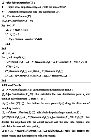

  

  The side lobe suppression algorithm based on background estimation

• (2) Define X _V as the max points along the direction of sampling number, from which the points larger than l _V are labeled as X _S .

• (3) Save the object regions between the two valley points around each point of X _S , calculate the correction factor d by the ratio between the max side lobe peak l _s and the max point l _m , then multiply the side lobe by d for offsetting.

As an illustration, a real multi-beam sonar image containing a metal cube tied with ropes is displayed in Fig. 9a. The sonar amplitude image is shown in Fig. 8a, with the size of 1024 (beam number) × 350(sampling number), and the corresponding normalized amplitude distribution is presented in Fig. 8b. As shown in Fig. 8b, the max distribution point l _m  = 0.62 and the max inflection point l _V  = 0.87 are obtained. The max amplitude for each sampling number is shown in Fig. 8c. As shown in Fig. 8c, the amplitude points X _S , which are larger than l _V (dashed line), including the highest points N (sampling number 250) are extracted from the X _V . For each point belonging to X _S , the object regions are saved while the side lobe regions are offset with the correction factor d. The object regions of N (between two dashed lines) and the max side lobe peak are shown in Fig. 8d. The l _s  = 0.86 derives the d = 0.72.

Fig. 8

An illustration of side lobe suppression algorithm. a Sonar amplitude image. b Normalized amplitude distribution. c The max amplitude for each sampling number. d Amplitude of sampling number 250

Local skewness images before and after side lobe suppression are displayed in Fig. 9b, c, using the computational window size T _W  = 14. The comparison reveals that a considerable improvement for object representation has been achieved with the proposed algorithm. The side lobes are reduced and the object regions are retained with a square structure.

Fig. 9

The side-lobe suppression algorithm for a multi-beam sonar image. a Original image. b Local skewness image before side lobe suppression. c Local skewness image after side lobe suppression

Another real multi-beam sonar image (shown in Fig. 12a) containing two groups of objects is used to compare the algorithms’ performance. Figure 10a shows the side lobe suppression with MVDR beamformer, and Fig. 10b shows the side lobe suppression with background estimation. It is clear that both the algorithms adequately reduce the side lobe. A significant SNR enhancement is achieved by the MVDR beamformer, whereas the boundary representations for potential objects are described in greater detail by the proposed algorithm. Furthermore, the proposed algorithm is about 200 times faster than the MVDR beamformer. This is a significant improvement in terms of real-time performance.

Fig. 10

Side lobe suppression using different algorithms. a MVDR beamformer algorithm. b The proposed algorithm

4 Results and discussion

The proposed approach is verified on several real sonar images, which were obtained from multi-beam sonar developed by Harbin Engineering University. The sonar covers a region of 140 (vertical) × 2.5 (horizontal), with an operating frequency of 300 kHz. The emitted signal is continuous wave (CW) with a pulse width of 0.1 ms, while the receiver is 64-element uniform linear array with a sampling frequency of 48 kHz. A large number of datasets collected during several trials are processed by beam forming and scan conversion methods [32–35], generating the image sequences with a resolution grid of 0.05 × 0.05 m², and two of them are selected for example in the following.

Dataset I was acquired from a trial at an indoor tank, Harbin Engineering University, China. The corresponding image sequence I has the size of 111 × 241 pixels. Each frame describes the water-column scenes of 7 × 10 m², in which a plastic ball and a metal block move together in horizontal direction. Two typical frames are presented in Fig. 11a, b, where the objects are hardly visible due to the small size and the similar amplitude of the object comparing to the background. The local skewness is estimated using the computational window size T _W  = 12, and the results are shown in Fig. 11c, d. Both the objects are represented with the square structure and distinguished from the background obviously. Table 5 gives the performance results, of which SNR ' is the SNR in local skewness image. The results show that local skewness image obtains the higher SNR ' and lower σ _B ', in contrast to original image.

Fig. 11

Local skewness for multiple objects representation in image sequence I. a Frame 1. b Frame 2. c Local skewness image for frame 1. d Local skewness image for frame 2

Dataset II was obtained from a trial at Songhua Lake, Jilin province, China. The corresponding image sequence II has the size of 361 × 601 pixels. Each frame describes the water-column scene of 20 × 30 m², in which two groups of objects move relatively in vertical direction. Each group of object is composed of a plastic ball and a metal block. A typical frame is displayed in Fig. 12a. Two groups of objects are distant, of which the object with low SNR can hardly be identified and the object with high SNR has high side lobes. Another frame is shown in Fig. 12b. Two groups of objects are close, of which the side lobes caused by high SNR objects occlude the other objects. After side lobe suppression, the local skewness is estimated using the computational window size T _W  = 14. The results are presented in Fig. 12c, d, where all objects are apparent with the square structure and the influence of side lobe are reduced. Table 6 gives the performance results. It shows that object 1 has a fluctuation of 11.87 dB between the original frames, whereas the corresponding fluctuation is only 1.99 dB between the local skewness frames. It confirms that local skewness is robust for object representation, especially in case of the object with a large SNR fluctuation between consecutive frames. Furthermore, the boundary of the high SNR object is distinct by implementing the proposed side lobe suppression algorithm.

Fig. 12

Local skewness for multiple objects representation in image sequence II. a Frame 1. b Frame 2. c Local skewness for frame 1. d Local skewness for frame 2

Table 5 Performance comparisons between the original image and local skewness image for partial frames of image sequence I

Table 6 Performance comparisons between the original image and local skewness image for partial frames of image sequence II

5 Conclusions

This paper investigates the capacity of local higher-order statistics (HOS) to represent objects in multi-beam sonar images. Local skewness is estimated using a sliding computational window applied to a sonar image, thus generating local skewness image of which a square structure is associated with a potential object. One finds that: (1) The Weibull distribution has been proved to be a better choice for modeling the background of multi-beam sonar image, by comparing with the log-normal and Rayleigh distributions. (2) The square structure composes of lower values in the middle, higher values on the edge, and the highest value in the corners, and makes the object easily identifiable. (3) Mapping from original image to local skewness image, an object with lower SNR achieves a higher object contrast C, whereas an object with higher SNR obtains a lower object contrast C, thus the robustness of object representation is improved, especially in case of the object with a large SNR fluctuation. (4) In order to select a suitable sliding computational window size, the α _min deriving from the size of computational window T _W should correspond to α ' for a highest h _T ; however, a trade-off between the higher skewness of object h _T and the lower standard deviation of background σ _B ' has to be made. (5) In the case of object with high SNR, an algorithm based on background estimation is able to significantly reduce the side lobe and completely retain object regions. The local HOS can provide the local feature relating to the potential object for segmentation, detection and classification tasks; however, the robustness of local feature should be further tested and improved for shape recognition. In the future, we plan to extend this work to multiple objects tracking in complex scenes.

References

SM Simmons, DR Parsons, JL Best, O Orfeo, SN Lane, R Kostaschuk, RJ Hardy, G West, C Malzone, J Marcus, P Pocwiardowski, Monitoring suspended sediment dynamics using MBES. J. Hydraul. Eng. 136(1), 45–49 (2010)
I Quidu, L Jaulin, A Bertholom, Y Dupas, Robust multitarget tracking in forward-looking sonar image sequences using navigational data. IEEE J. Ocean. Eng. 37(3), 417–430 (2012)
GG Acosta, SA Villar, Accumulated CA–CFAR process in 2-D for online boject detection from sidescan sonar data. IEEE J. Ocean. Eng. 40(3), 558–569 (2015)
XF Ye, ZH Zhang, PX Liu, HL Guan, Sonar image segmentation based on GMRF and level-set models. Ocean Eng. 37(10), 891–901 (2010)
T Celik, T Tjahjadi, A novel method for sidescan sonar image segmentation. IEEE J. Ocean. Eng. 36(2), 186–194 (2011)
RJ Campbell, PJ Flynn, A survey of free-form object representation and recognition techniques. Comput. Vis. Image Underst. 81(2), 166–210 (2001)
B Moghaddam, A Pentland, Probabilistic visual learning for object representation. IEEE Trans. Pattern Anal. Mach. Intell. 19(7), 786–793 (2005)
D Dai, MJ Chantler, DM Lane, N Williams, Proceedings of International Conference on Image Processing and Its Applications. A spatial-temporal approach for segmentation of moving and static objects in sector scan sonar image sequences, 1995, pp. 163–167
JP Stitt, RL Tutwiler, AS Lewis, Proceedings of the IASTED International Conference on Signal and Image Processing. Fuzzy c-means image segmentation of side-scan sonar images, 2001, pp. 27–32
M Mignotte, C Collet, P Perez, P Bouthemy, Sonar image segmentation using an unsupervised hierarchical MRF model. IEEE Trans. Image Process. 9(7), 1216–1231 (2000)
GJ Dobeck, JC Hyland, L Smedley, Proceedings of the International Society for Optical Engineering (SPIE). Automated detection/classification of sea mines in sonar imagery, 1997, pp. 90–110
S Reed, Y Petillot, J Bell, Model-based approach to the detection and classification of mines in sidescan sonar. Appl Opt 43(2), 237–246 (2004)
DP Williams, Bayesian data fusion of multiview synthetic aperture sonar imagery for seabed classification. IEEE Trans. Image Process. 18(6), 1239–1254 (2009)
CM Ciany, W Zurawski, Proceedings of Oceans Mts/IEEE Conference & Exhibition. Performance of computer aided detection/computer aided classification and data fusion algorithms for automated detection and classification of underwater mines, 2001, pp. 277–284
S Reed, IT Ruiz, C Capus, Y Petillot, The fusion of large scale classified side-scan sonar image mosaics. IEEE Trans. Image Process. 15(7), 2049–2060 (2006)
GR Cutter Jr, Y Rzhanov, LA Mayer, Automated segmentation of seafloor bathymetry from multibeam echosounder data using local Fourier histogram texture features. J. Exp. Mar. Biol. Ecol. 285(2), 355–370 (2003)
A Mahiddine, J Seinturier, JM Boï, P Drap, D Merad, Proceedings of 20th International Conference on Computer Graphics, Visualization and Computer Vision. Performances Analysis of Underwater Image Preprocessing Techniques on the Repeatability of SIFT and SURF Descriptors, 2012, pp. 275–282
S Lyu, H Farid, Steganalysis using higher-order image statistics. IEEE Trans. Inf. Forensic Secur. 1(1), 111–119 (2006)
A Briassouli, I Kompatsiaris, Robust temporal activity templates using higher order statistics. IEEE Trans. Image Process. 18(12), 2756–2768 (2009)
F Maussang, J Chanussot, A Hetet, M Amate, Higher-order statistics for the detection of small objects in a noisy background application on sonar imaging. EURASIP J. Adv. Signal Process. 2007(1), 1–17 (2007)
F Maussang, J Chanussot, A Hetet, M Amate, Mean–standard deviation representation of sonar images for echo detection: application to SAS images. IEEE J. Ocean. Eng. 32(4), 956–970 (2007)
S Kuttikkad, R Chellappa, Proceedings of IEEE International Conference on Image Processing. Non-Gaussian CFAR techniques for target detection in high resolution SAR images, 1994, pp. 910–914
JM Gelb, RE Heath, GL Tipple, Statistics of distinct clutter classes in midfrequency active sonar. IEEE J. Ocean. Eng. 35(2), 220–229 (2010)
DA Abraham, JM Gelb, AW Oldag, Background and clutter mixture distributions for active sonar statistics. IEEE J. Ocean. Eng. 36(2), 231–247 (2011)
IR Joughin, DB Percival, DP Winebrenner, Maximum likelihood estimation of K distribution parameters for SAR data. IEEE Trans. Geosci. Remote Sens. 31(5), 989–999 (1993)
DR Iskander, AM Zoubir, B Boashash, A method for estimating the parameters of the K distribution. IEEE Trans. Signal Process 47(4), 1147–1151 (1999)
M Mignotte, C Collet, P Pérez, P Bouthemy, Three-class Markovian segmentation of high-resolution sonar images. Comput.Vis.Image.Und 76(3), 191–204 (1999)
DN Joanes, CA Gill, Comparing measures of sample skewness and kurtosis. J.R.Stat.Soc 47(1), 183–189 (1998)
JF Synnevag, A Austeng, S Holm, A low-complexity data-dependent beamformer. IEEE Trans. Ultrason. Ferroelectr. Freq. Control 58(2), 281–289 (2011)
CC Gaudes, I Santamaría, J Vía, EM Gómez, TS Paules, Robust array beamforming with sidelobe control using support vector machines. IEEE Trans. Signal Process. 55(2), 574–584 (2007)
M Wax, Y Anu, Performance analysis of the minimum variance beamformer. IEEE Trans. Signal Process 44(4), 928–937 (1996)
C Xu, HS Li, BW Chen, T Zhou, Multibeam interferometric seafloor imaging technology. J. Harbin Eng. Univ. 34(9), 1159–1164 (2013)
X Liu, HS Li, T Zhou, C Xu, B Yao, Multibeam seafloor imaging technology based on the multiple sub-array detection method. J. Harbin Eng. Univ. 33(2), 197–202 (2012)
A Trucco, M Garofalo, S Repetto, G Vernazza, Processing and analysis of underwater acoustic images generated by mechanically scanned sonar systems. IEEE Trans. Instrum. Meas. 58(7), 2061–2071 (2009)
R Schettini, S Corchs, Underwater image processing: state of the art of restoration and image enhancement methods. EURASIP J. Adv. Signal Process. 2010(3), 1–14 (2010)
Acknowledgements
This work was supported by the National Natural Science Foundation of China (Grant No. 41327004, 41376103, 41306038, and 41506115) and the Fundamental Research Funds for the Central Universities (Grant No. HEUCF160510). The authors would like to thank the anonymous reviewers for the constructive comments on the manuscript.
Competing interests
The authors declare that they have no competing interests.
Author information
Authors and Affiliations
Corresponding author
Additional information
An erratum to this article is available at http://dx.doi.org/10.1186/s13634-017-0471-2.
Rights and permissions
Open Access This article is distributed under the terms of the Creative Commons Attribution 4.0 International License (http://creativecommons.org/licenses/by/4.0/), which permits unrestricted use, distribution, and reproduction in any medium, provided you give appropriate credit to the original author(s) and the source, provide a link to the Creative Commons license, and indicate if changes were made.
About this article
Cite this article
Li, H., Gao, J., Du, W. et al. Object representation for multi-beam sonar image using local higher-order statistics. EURASIP J. Adv. Signal Process. 2017, 7 (2017). https://doi.org/10.1186/s13634-016-0439-7
Received:
Accepted:
Published:
DOI: https://doi.org/10.1186/s13634-016-0439-7