- Research
- Open access
- Published:
Multiple importance sampling revisited: breaking the bounds
EURASIP Journal on Advances in Signal Processing volume 2018, Article number: 15 (2018)
Abstract
We revisit the multiple importance sampling (MIS) estimator and investigate the bound on the efficiency improvement over balance heuristic estimator with equal count of samples established in Veach’s thesis. We revise the proof for this and come to the conclusion that there is no such bound and henceforth it makes sense to look for new estimators that improve on balance heuristic estimator with equal count of samples. Next, we examine a recently introduced non-balance heuristic MIS estimator that is provably better than balance heuristic with equal count of samples, and we improve it both in variance and efficiency. We then obtain an equally provably better one-sample balance heuristic estimator, and finally, we introduce a heuristic for the count of samples that can be used when the individual techniques are biased. All in all, we present three new sampling strategies to improve on both variance and efficiency on the balance heuristic using non-equal count of samples.
Our scheme requires the previous knowledge of several quantities, but those can be obtained in an adaptive way. The results also show that by a careful examination of the variance and properties of the estimators, even better estimators could be discovered in the future. We present examples that support our theoretical findings.
1 Introduction
The multiple importance sampling (MIS) estimator [1, 2], and in particular balance heuristic, which is equivalent to the Monte Carlo estimator with a mixture of probability density functions (pdfs), has been used for many years with a big success, being a reliable and robust estimator that allows an easy and straightforward combination of different sampling techniques. MIS with balance heuristic estimator has been almost exclusively used with equal count of samples for each technique, mainly following the recommendations based on certain quasi-optimality theorems in Veach’s thesis. Specifically, these theorems stated that a balance heuristic estimator could not be worse than n times any other MIS estimator with equal count of samples where n is the number of combined methods. In papers addressing the variance of MIS, strategies were assumed to have equal number of samples [3, 4], and the combination of MIS with jittered sampling was studied in [5].
MIS is often used in rendering applications of computer graphics [6] where the reflected illumination is the product of the intensity in the illumination direction that can be represented by an environment map, and the probability of the reflection from a surface. As it is not feasible to sample with this product of two functions, sampling mimics either directions from where reflection is likely or directions of high intensity. The first approach is called light source sampling and the second approach is called BRDF sampling after the name of the bidirectional reflection distribution function (BRDF).
Lu et al. [7] propose an improvement to balance heuristic estimators for environment map illumination by using a Taylor’s second order approximation of the variance around the equal weights 1/2 to obtain the counts of samples according to the BRDF and the environment map, which is accurate only if the optimal sample numbers are not too far from equal sampling. Heuristics have also been used that prefer certain sampling methods based on the local properties, for example, BRDF sampling is advantageous on highly specular surfaces and light source sampling on diffuse surfaces. Pajot et al. proposed a framework, called representativity, to develop such heuristic [8]. Havran and Sbert [9, 10] introduce a heuristic for unbiased techniques based on assigning a count of samples proportional to the inverse of the variance of each technique that in some cases seemed to put into question the quasi-optimality rules of equal sampling. More recently, based on the analysis of the variance of MIS estimators, Sbert et al. [11] discovered a MIS non-balance heuristic estimator that is provably better than balance heuristic with equal count of samples. The introduction of costs into those schemes allowed an even bigger increase in efficiency. We improve on their work by clarifying the quasi-optimality rules in Veach’s thesis by introducing new balance heuristic estimators that are provably better than balance heuristic with equal count of samples, and by introducing a new heuristic valid when the individual estimators are biased. We believe that our work can inspire new provably better estimators or at least sound heuristics for heuristically better estimators.
Putting our results in a wider perspective, we should consider adaptive variance reduction methods that learn some properties of the integrand, e.g., the location of its peak, and refine the sampling strategy on-the-fly by analyzing the samples that have been already generated. In case of mixing different pdfs with which sampling is straightforward, the weights of the individual methods are the target of the adaptation. Adaptive methods can be imagined as a sequence of Monte Carlo quadrature steps and parameter estimation steps. Care should be exercised to implement adaptive methods since making the sampling pdf dependent on the generated samples might make the estimator biased, which can be attacked by freezing the adaptation after certain samples letting the approach be consistent. Another challenge is the control of the adaptation with randomly sampled, i.e., noisy data. To handle this, adaptive MCMC approaches often choose an artificial but robust criterion, like the acceptance rate, instead of the variance of the estimation [12, 13]. In computer graphics, this technique has been used to control the mutation of MCMC methods [14, 15] and to distribute different numbers of samples among the different techniques [16].
Owen and Zhou [17] survey the principles of adaptively mixing different sampling strategies, including defensive importance sampling and the simultaneous application of control variates and importance sampling. They also investigate MIS and point out that there is a room for improvement. Douc et al. [18] investigated the population Monte Carlo method and derived sufficient convergence conditions for adaptive mixtures, and also iterative formulae for the optimal weights [19]. As population Monte Carlo explores the sampling space with a Markov stochastic process, it uses the information of only the current samples directly. Cornuet et al. [20] improve this in their adaptive multiple importance sampling algorithm and present optimal exploitation of previous samples, which automatically stabilizes the process. Marin et al. [21] argue that the Markov property is important to be able to prove the consistency of the estimator, and the stability of the process can be achieved by increasing the sample size in each iteration.
In their recent work, Martino, Elvira et al. proposed adaptive population importance sampling [22] and gradient adaptive population importance sampling [23] that adapt the mean and the covariance of proposal Gaussian pdfs, and reported significant improvements with respect to MIS that keeps the individual proposal pdfs fixed. We note that in computer graphics the not continuous integrands may pose problems to such gradient-based methods. Elvira et al. also examined a discrete weighting scheme [24] where only a subset of available sampling strategies is selected with the aim of reducing the computational complexity of the sampling process.
The rest of the paper is organized as follows: In Section 2, we review the basic formulae for the variance of MIS. In Section 3, we discuss Theorem 9.5 of Veach’s thesis and present a new proof for a slightly modified theorem. In Section 4, we present a multi-sample balance heuristic estimator that is provably better than multi-sample balance heuristic with equal count of samples. In Section 5, we obtain a provably better one-sample balance heuristic estimator, and in Section 6, we justify a new heuristic for the count of samples that does not require the individual techniques be unbiased. In Section 7, we discuss the results, and in Section 8, summarize our conclusions. Some proofs are given in Appendices A and B, and numeric 1D examples are presented in Appendix C.
2 MIS variance analysis
We review here the variance of MIS estimators. The naming convention for the estimators is given in Table 1.
2.1 General multi-sample MIS estimator
The MIS estimator introduced by Veach and Guibas [1] to estimate the value of integral \(I = \int f(x) {\mathrm d} x\) has the following form:
where the weights w i (X ij ) are such that
and
In this combination scheme, sampling method i uses probability density function p i (x) to generate N i number of random samples {X ij }, (j=1,…,N i ). If we have n techniques, the total number of samples is \(\sum _{i=1}^{n} N_{i} =N\). Integral estimator F is unbiased, as its expected value μ is equal to integral I:
The variance of the estimator is given in the proof of Theorem 9.2 of Veach’s thesis [2]. Define F ij as
For a fixed method i and all j values, the estimators {F ij } are independent identically distributed random variables with expected value μ i :
Observe that
and that the variance of F ij is
If samples are statistically independent, the variance of the integral estimator is
There are two different components of a MIS estimator that determine the variance of the estimates: weighting scheme w i and the number of samples N i allocated to different methods. Weighting functions may or may not depend on the number of samples. Additionally, the number of samples can be pre-determined, called the multi-sample model, or selected also randomly, which leads to the one-sample model.
2.2 Balance heuristic estimator
Veach defined a balance heuristic estimator setting the weights as the following:
These weights lead to the following estimator:
Let us now consider the variance of the combined estimator when method i takes N i samples and predetermining the number of samples in advance (multi-sample model):
where α k =N k /N.
2.2.1 Balance heuristic with equal count of samples
Observe that if we take equal count of samples for each technique, i.e., for all i, N i = N/n or α i = 1/n, then the weights become
the estimator is
and the variance is equal to
where \(\sigma ^{2}_{i,{\text {eq}}}\) is equal to
and μi,eq is
2.3 A provably better non-balance heuristic estimator
Sbert et al. [11] introduced an estimator provably better than balance heuristic with equal count of samples. Taking the weights as in Eq. 14, the estimator F in Eq. 1 is
The estimators F ij in Eq. 5 become
and the variances \(\sigma ^{2}_{i}\) defined by Eq. 9 are equal to \(\sigma ^{2}_{i,{\text {eq}}}\). The variance, Eq. 10, is then
Sbert et al. showed [11] that taking N i ∝σi,eq guarantees that we improve on balance heuristic with equal sampling by using estimator Eq. 19, up to the statistical error in estimating the σi,eq values.
Taking into account the cost c i of sampling with technique i, the sample numbers that guarantee that we improve the efficiency (i.e., the inverse of cost times variance) over balance heuristic with equal sampling are
3 Breaking the bounds for the relative acceleration
In this section, we investigate the bounds for the improvement on the variance of balance heuristic estimator with equal count of samples.
This problem has been attacked by Veach establishing an inequality (Theorem 9.5 of his thesis [2]) for the variance of the balance heuristic estimator with equal count of sampling \({\hat F}_{{\text {eq}}}\):
where F is any multiple importance sampling estimator using the same total number of samples N. Veach interpreted Theorem 9.5 as a proof of quasi-optimality of balance heuristic with equal count of samples, saying “According to this result, changing the N i can improve the variance by at most a factor of n, plus a small additive term. In contrast, a poor choice of the w i can increase variance by an arbitrary amount. Thus, the sample allocation is not as important as choosing a good combination strategy.”
The proof of Eq. 23 is based on the following inequality, which compares a general multiple importance sample estimator F with arbitrary number of samples {N i } with the same estimator (i.e., using the same weights w i ) but with equal count of samples, Feq as follows:
But this inequality is not valid when the weights w i (x) depend on the number of samples N i , see Appendix A for a proof. Just to give a single counter example, let us consider the case when zero variance estimator is possible by properly setting the number of samples, making V[F] zero, but the equal count of samples estimator will not have zero variance. However, we show that Theorem 9.5 can be generalized to such cases as well, but it requires the full reconsideration of the original proof.
The interpretation by Veach of Theorem 9.5 is based on the assumption that additive term μ2(n−1)/N is small if the total number of samples, N, gets larger. However, denominator N is implicitly included in the other terms of Eq. 23 as well, thus the considered additive term is, in fact, not negligible. As a result, the selection of N i sample numbers or weights α i can make a significant difference in the variance, which is worth examining and opens possibilities to find better estimators.
3.1 One-sample balance heuristic
The general MIS one-sample primary estimator is
where technique i is selected with probability α i . It can be easily shown that it is unbiased, i.e., its expected value is μ. Using the balance heuristic weights,
the estimator becomes the one-sample balance heuristic estimator,
One-sample balance heuristic is the same as the Monte Carlo estimator using the mixture of probabilities \(p(x)~=~\sum _{k~=~1}^{n} \alpha _{k} p_{k}(x)\), \(\sum _{k~=~1}^{n} \alpha _{k}~=~1\). The α i values are called the mixture coefficients and represent the average count of samples from each technique. The variance of this estimator can be obtained by the application of the definition of variance,
Theorem 1
If \(V\left [\!\hat {\mathcal {F}}_{{\text {eq}}}^{1}\right ]\) is the variance of the one-sample balance heuristic estimator with equal weights, and \(V\left [\!\hat {\mathcal {F}}^{1}\right ]\) the variance of the one-sample balance heuristic estimator with any distribution of weights {α k }, then the following inequality holds:
Proof
The variance of the one-sample balance heuristic with equal weights is
As \(\alpha _{\max } \sum _{k=1}^{n} p_{k}(x) \ge \sum _{k=1}^{n} \alpha _{k} p_{k}(x)\) where αmax>0 is the maximum of the values of α k and p k is not negative, we have \(\frac {1}{n} \alpha _{\max } \sum _{k=1}^{n} p_{k}(x) \ge \frac {1}{n} \sum _{k=1}^{n} \alpha _{k} p_{k}(x)\) and thus:
□
When for all i, α i =1/n, Eq. 29 becomes an equality.Observing that αmax≤1, the following corollary is immediate.
Corollary 1
Equations 29 and 32 do not imply that the improvement with respect to the equal count of samples is limited by a factor of n, since μ can be large in comparison with the variances. So, it is worth trying to obtain α i values that can reduce the variance.
Equations 29 and 32 can be extended to the one-sample MIS in general using Theorem 9.4 of Veach’s thesis, which states that the variance of the one-sample MIS estimator is minimal when it is a balance heuristic one, i.e., \(V[\hat {\mathcal {F}}] \le V[{\mathcal {F}}]\). For instance, for Eq. 32
And for N samples,
Observe that Eq. 34 is similar to Eq. 23 except for the fact that it holds for the one-sample estimator. Using \(V[\!\hat {F}] \le V[\!\hat {\mathcal {F}}]\) (as shown in [11]) we also have:
Finally, note that we do not state that Eq. 23 is invalid, but that its proof by Veach in his thesis [2] is wrong and also his interpretation is not correct. On the other hand, we have proved a formally identical relationship, Eq. 34, for the one-sample MIS estimator instead of the multi-sample estimator.
4 A provably better balance-heuristic multi-sample estimator
In Section 1, we reviewed two strategies for the allocation of samples to individual methods, balance heuristic with equal count of samples (Section 2.2.1) and non-balance heuristic with sample numbers proportional to the variance (Section 2.3). The variance of the latter is better than that of the equal count estimator. This section shows that we can do it even better if the sample allocation strategy of Section 2.3 is applied to balance heuristic.
We can use Theorem 9.2 from Veach’s thesis, which states that for any MIS estimator F, the balance heuristic estimator \(\hat {F}\) with the same count of samples as F has always less variance up to an asymptotically decreasing factor, i.e.,
to obtain a provably better estimator than the one described in Section 2.3. Let us now take the estimator F as Eq. 19 from Section 2.3 where N i ∝σi,eq. This is provably better than the balance heuristic with equal count of samples, \(\hat {F}_{{\text {eq}}}\), i.e., \(V[{F}] \le V[\hat {F}_{{\text {eq}}}]\). Thus,
Observe that \(\hat {F}\) is the balance heuristic estimator defined in Eq. 12 where the N i ∝σi,eq. Similar results can be obtained for the case when the sampling cost is also taken into account, i.e. consider now as F the MIS estimator with \(N_{i} \propto {\sigma _{i,{\text {eq}}}}/{\sqrt {c_{i}}}\).
Estimator \(\hat {F}\) is now the balance heuristic estimator defined in Eq. 12 with \(N_{i} \propto {\sigma _{i,{\text {eq}}}}/{\sqrt {c_{i}}}\).
4.1 Discussion
Let us re-write Eq. 37 with variances \(V_{1}[\!\hat {F}], V_{1}[\!{F}]\), and \(V_{1}[\!\hat {F}_{{\text {eq}}}]\) normalized to N = 1, i.e., \(V[\!\hat {F}]=V_{1}[\!\hat {F}]/N, V[\!{F}]~=~V_{1}[\!{F}]/N, V[\!\hat {F}_{{\text {eq}}}]~=~V_{1}[\!\hat {F}_{{\text {eq}}}]/N\):
The efficiency in this case is
Thus, the relative difference between variances will be constant disregarding N. This is a similar situation to that encountered in Section 3.
5 A provably better one-sample balance heuristic estimator
The variance of the estimator in Eq. 25 is the second moment minus the square of μ:
where the second moments \(M_{i}^{2}\) are defined as
Observe that, as μ2 is a constant, minimizing \(V[{\mathcal {F}}^{1}]\) means minimizing the first term of the last equality in Eq. 41. When the weights {w i (x)} are independent of the coefficients {α i }, we get the following theorem:
Theorem 2
When the weights {w i (x)} are independent of the {α i }, the minimum variance in Eq. 41 is obtained when
Proof
The proof fully given in Appendix B follows from applying the Lagrange multipliers method to the target function:\(\Lambda (\alpha _{i}, \lambda)=\sum _{i=1}^{n} \frac {1}{\alpha _{i}} M_{i}^{2} - \mu ^{2} + \lambda \left (\sum _{k=1}^{n} \alpha _{k} -1\right)\). □
Let us use the weights of Section 2.3, i.e., \(w_{i}(x) = {p_{i}(x)}/{\sum _{k=1}^{n} p_{k}(x)}\). These weights do not depend on the {α i }, and thus we can apply Theorem 2. The minimum variance is then given by substituting the optimal {α i } from Eq. 43 to Eq. 41, resulting in
where the Mi,eq values are the square root of
obtained by substituting the weights of Section 2.3 into Eq. 42. As they correspond to the minimum variance, the values obtained in Eq. 43 will provide a variance less than using any other count of samples, in particular when taking equal count of samples, thus we get
Observe that the right side in Eq. 46 also corresponds to the variance of the one-sample balance heuristic estimator with equal count of samples, i.e., for all i, α i = 1/n. Thus, we can guarantee that the one-sample estimator given by Eq. 25 using weights of Section 2.3 is better than the one-sample balance heuristic estimator with equal count of samples. Applying now Theorem 9.4 of Veach’s thesis, that reads
we have that the one-sample balance heuristic estimator
using α i ∝Mi,eq weights is guaranteed to have less variance than the one-sample balance heuristic estimator with equal count of samples. If we take into account the costs, we have the following theorem:
Theorem 3
When the weights {w i (x)} are independent of the {α i }, the maximum efficiency of MIS one-sample estimator is obtained when
See Appendix B for a proof. Observe, however, that Eq. 49 is not an explicit expression for α i since it contains these values in the right hand side, as \(C_{T} = \sum _{k~=~1}^{n} \alpha _{k} c_{k}\). Thus, some approximation is needed in practice. One possibility is to take
another is to substitute in the right side of Eq. 49 the optimal values independent of the costs, i.e., α i ∝M i . Under certain circumstances, we can guarantee that the one-sample balance heuristic estimator using the values
is more efficient than the one-sample balance heuristic with equal count of sampling.
Theorem 4
The one-sample balance heuristic estimator using the {α i } values in Eq. 51 is more efficient than the one-sample balance heuristic estimator with equal count of sampling when the {α i } values are decreasing with costs {c i }.
A proof can be found in Appendix B. The estimator would be now
When the variation of Mi,eq values is small relatively to the variation of c i values, then we can consider that \(\alpha _{i} \propto {M_{i,{\text {eq}}}}/{\sqrt {c_{i}}}\) values are decreasing with c i , and the efficiency of MIS estimator using \(\alpha _{i} \propto {M_{i,{\text {eq}}}}/{\sqrt {c_{i}}}\) would be better than taking α i = 1/n.
5.1 Discussion
One might ask why we are interested in the one-sample estimator when its variance is always higher than its multi-sample version due to the additional randomization. In addition, as the costs C T are the same, as we use on average the same number of samples from each technique for both the one-sample and the multi-sample estimators, we also have \(C_{T} V[\!{F}] \le C_{T} V[\!\mathcal {F}]\), this is, given a one-sample estimator, its corresponding multi-sample counterpart will always be more efficient. However, there might be cases where only the one-sample estimator is applicable, e.g., when we do not know a priori the number of samples or we need just a single sample.
6 A new heuristic
In [9, 10] the heuristic α i ∝1/v i was presented, where \(v_{i}=\int \frac {f^{2}(x)}{p_{i}(x)} {\mathrm {d}}x- \mu ^{2}\) is the variance of technique i. This heuristic is only valid when all techniques p i (x) are unbiased. We will present here a generalized heuristic that is valid even when the techniques are biased and based on the following theorems.
Theorem 5
The variance \(V[\hat {\mathcal {F}}^{1}]\) is bounded by
where \(m_{k}^{2} = \int \frac {f^{2}(x)}{p_{k}(x)} {\mathrm {d}}x\) is the second moment of technique k.
Proof
Using the inequality between harmonic and arithmetic means, we get
Observe that we do not require the {p k } techniques be unbiased. □
If all techniques are unbiased, then
which follows from that μ2 can be written as \(\sum _{k} \alpha _{k} \mu ^{2}\). Note that from \(V[\!\hat {F}] \le V[\!\hat {\mathcal {F}}]\), the bound in Eqs. 53 and 55 also holds for \(V[\!\hat {F}]\).
Observe also that if \(m_{\max }^{2} = \max _{k} \left \{m_{k}^{2}\right \}\) and \(v_{\max } = \max _{k}^{2} \{v_{k}\}\), then from Eq. 53
and in case of unbiased techniques from Eq. 55
That is, whichever combination {α k } is taken, we cannot make it worse than just using the worst technique.
Let us use Theorem 5 to obtain a heuristic valid for biased techniques.
Theorem 6
Consider a function f(x) and n not necessarily unbiased Monte Carlo integration techniques, {p i (x)}, with second moments \(\left \{m_{i}^{2}\right \}\), and the sequence of n positive values {α i }, \(\sum _{i} \alpha _{i}=1\). The rearrangement that minimizes the bound in Eq. 53 happens when the {α i } are ordered inversely to \(\left \{m_{i}^{2}\right \}\).
Proof
As μ is a constant value only depending on f(x), the rearrangement that minimizes the bound in Eq. 53 is the one that minimizes \(\sum _{k=1}^{n} \alpha _{k} m_{k}^{2}\), and by virtue of the rearrangement inequality [25, page 261][26], it happens when the {α i } are ordered inversely to \(\left \{m_{i}^{2}\right \}\). □
Theorem 6 justifies the introduction of the new heuristic \(\alpha _{i} \propto {1}/{m_{i}^{2}}\). We can extend this heuristic to take the costs of the techniques into account, in the same way as in [9] and [10] by using \(\alpha _{i} \propto {1}/{\left (c_{i} m_{i}^{2}\right)}\).
7 Results
7.1 1D functions
We have compared the following estimators: equal count of samples with balance heuristic, count inversely proportional to variances of independent techniques with balance heuristic [9, 10], optimal count non-balance heuristic in [11], and the new balance heuristic estimators defined in Sections 4, 5, and 6 using values α k ∝σk,eq,α k ∝Mk,eq, and \(\alpha _{k} \propto \frac {1}{m^{2}_{k}}\) for equal cost of sampling, and \(\alpha _{k} \propto \frac {\sigma _{k,eq}}{\sqrt {c_{k}}}, \alpha _{k} \propto \frac {M_{k,eq}}{\sqrt {c_{k}}}\), and \(\alpha _{k} \propto \frac {1}{c_{k} m^{2}_{k}}\) for unequal cost of sampling. The new estimators are tried for both the one-sample and the multi-sample case. The results for 1D example functions and pdfs of Fig. 1 are presented in Appendix C and summarized in Tables 2, 3, 4, 5, and 6. We additionally provide in supplemental material the Mathematica code to try any function with any pdfs. In the obtained results, we can see the following patterns:
-
As expected [11] multi-sample estimators are always better than the corresponding one-sample estimators with the same distribution of samples
Fig. 1 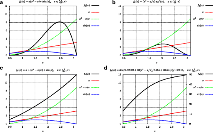
From left to right and from top to bottom: The four functions (in black) used in the four examples, f1(x) (example 1), f2(x) (example 2), f3(x) (example 3), f4(x) (example 4), as combination of the three functions x (red), x2−x/π(green), and sin(x) (blue)
Table 2 Variances for multi-sample estimator for the four examples in Appendix C and the environment map example (× 10−3) for balance heuristic using equal count of samples, for the count inversely proportional to the variances of independent estimators [9] and [10], for the provably better, non-balance heuristic, estimator defined in [11], and for the three new estimators defined in this paper Table 3 Variances for one-sample balance heuristic for the four examples in Appendix C and the environment map example (× 10−3) for balance heuristic using equal count of samples, for the count inversely proportional to the variances of independent estimators [9] and [10], and for the three new estimators defined in this paper Table 4 Variance times cost (i.e., inefficiency, the smaller the better) for multi-sample estimator for the four examples in Appendix C and the environment map example (× 10−3) for balance heuristic using equal count of samples, for the count inversely proportional to the variances of independent estimators [9] and[10], for the provably better, non-balance heuristic, estimator defined in [11], and for the three new estimators defined in this paper Table 5 Variance times cost (i.e., inefficiency, the smaller the better) for one-sample estimator for the four examples in Appendix C and the environment map example (× 10−3) for balance heuristic using equal count of samples, for the count inversely proportional to the variances of independent estimators [9] and[10], and for the three new estimators defined in this paper Table 6 \(\alpha _{i}^{j}\): α i values for the j-th 1D example and for the environment map example -
As expected the multi-sample estimators defined in [11] (Section 2.2.1) are better than balance heuristic with equal count of samples, both in variance and efficiency.
-
The new multi-sample estimators defined in Section 4 have similar variance values than balance heuristic with equal number of samples, but have better values for efficiency, both for the one-sample and the multi-sample estimator.
-
The new multi-sample estimators defined in Section 4 provide similar variance as the ones in [11] but better efficiency, except in the fourth example where the efficiency is slightly worse.
-
The optimal distribution of samples obtained in Section 5 performs always better for both the one-sample and the multi-sample estimator cases than the balance heuristic estimator with equal count of samples, in both variance and efficiency. This improvement is notable, especially when we consider that example 4 is particularly well suited for the equal count of sampling.
-
The multi-sample estimators using the optimal distribution of samples obtained in Section 5 perform better than the multi-sample estimators defined in [11], in both variance and efficiency.
-
The heuristically based estimators defined in [9] and in Section 6 give the best results for the first three examples, but are by far the worst for the fourth example.
-
The heuristically based estimators for unbiased techniques defined in [9] and [10] give better results than the one defined in Section 6 for possibly biased techniques, except for the third example, where the new heuristic performs much better.
-
We obtain in one case an acceleration of more than 30 times over the variance of the balance heuristic estimator with equal count of samples.

7.2 Adaptive results for 1D functions
We present also results for the four 1D examples computed with adaptive sampling algorithms. A first batch using equal number of samples from each technique computes order 1 approximation of the different quantities, which in turn allows us to obtain a first approximation of the α values needed for the second batch. The samples of batch \({\mathcal {N}}+1\) are obtained with the order \({\mathcal {N}}\) approximation of the α values, and incrementally update the \({\mathcal {N}}\)-order quantities. We provide in supplemental material the C++ code to compute all estimators adaptively. The pseudo-code for the estimators defined in [9] and [10] can be found in the supplementary material of [10]. The charts with variances normalized to 1 sample, (i.e., variance times the number of samples), and variances times cost (i.e., inefficiencies) for specific costs as described in the Appendix C, and averaged for 100 runs are shown in Figs. 2 and 3 for samples count from 35 to 5000.

The variance for the estimators for adaptive sampling for different samples count and unit cost of sampling techniques. a Example 1, b example 2, c example 3, and d example 4. Notation of lines 1 to 6 used in charts follows the order of row in Table 2

7.3 2D analytical environment map example with Lafortune-Phong BRDF model
Let us consider here the BRDF formula for the physically based variant of the Phong model presented by Lafortune [27], assuming the case when the outgoing direction ω o is the surface normal:
where ρ d is the diffuse albedo, ρ s is the specular albedo, m is the shininess, and θ is the angle between incident direction ω i and the surface normal.
Let us consider also an environment map of intensity R(ω i )=R· cosθ. As dω= sinθdθdϕ the outgoing radiance is given then by the integral for the hemisphere in spherical parametrization θ,ϕ of the incident direction
and integrating over ϕ we get
By the variable substitution of x= cosθ, we obtain
We have thus the integral of the product p1(x)p2(x), where p1(x) corresponds to the BRDF times x= cosθ,
and p2(x)=x is the environment map.
We used typical values, m = 5, ρ d = ρ s = 0.5, and compared for equal cost and for the empirically obtained sampling costs, c1 = 1,c2 = 4.8. The detailed results are in the last columns of Tables 2, 3, 4, 5, and in the last two columns of Table 6. The results confirm the patterns found in our 1D examples.
8 Conclusions
This paper discussed an important topic of MIS estimators and the limited acceleration over equal count of samples balance heuristic. We have shown that in reality, this bound on acceleration does not hold, which justifies the search for better and more efficient estimators. We have obtained, both without and with taking into account the cost of sampling, new balance heuristic estimators that are provably better than balance heuristic with equal count of samples, and new heuristic estimators valid even when the independent techniques are biased. We have analyzed their behavior with 1D examples and with a 2D environment map example.
9 Appendix A: Inequality in Theorem 9.5 of Veach’s thesis does not hold for balance heuristic
Let us repeat first the proof of Eq. 24 such as it appears in Veach’s thesis
where V[ Feq] is computed assuming the same weights as V[ F] but with equal count of samples. Let us see that inequality 61 does not hold when the weights w i (x) depend on the N i . We will see it for the balance heuristic estimator, where the weights are defined by
Eq. 61 would be
as the last but two expression is clearly not the variance of a balance heuristic estimator with equal count of samples (Eq. 16). Inequality 61 thus holds only when the weights w i (x) do not depend on counts N i , and thus the proof of Theorem 9.5 is not valid in this case.
10 Appendix B: Section 5 proofs
We present the proof of Theorem 2. This proof is similar to the proof of Theorem 2 in [11].
Proof
To optimize the variance \(V\big [\!\hat {\mathcal {F}^{1}}\big ] \,=\, \sum _{i=1}^{n} \frac {1}{\alpha _{i}} M^{2}_{i}-\mu ^{2}\), we use Lagrange multipliers with the constraint \(\sum _{i=1}^{n} \alpha _{i} = 1\) and objective function
Computing the partial derivatives and equating them to zero, as the M i do not depend on the α i , we get
Thus for all j values \(\lambda = {M^{2}_{j}}/{\alpha _{j}^{2}}\), which implies that α j ∝M j . The Hessian matrix, obtained with the second derivatives of \(V[\hat {\mathcal {F}^{1}}]\), is a diagonal matrix with positive diagonal values
and thus is positive-definite. The variance function is then strictly convex in its convex domain \(\sum _{i=1}^{n} \alpha _{i} = 1\), where for all i, 0<α i <1, meaning that the critical point is unique and a minimum.
Substituting the optimal values, i.e., α j ∝M j , we find the minimum variance,
□
We present now the proof of Eq. 49.
Proof
Let us consider c i the cost of sampling with technique i. The average cost (or cost for one total sample) is thus \(C_{T} = \sum _{i} \alpha _{i} c_{i}\). We want to minimize now the cost times variance, i.e., \(C_{T} \times V\left [\!{\mathcal F}^{1}\right ]\), which is the inverse of efficiency. We use Lagrange multipliers with the constraint \(\sum _{i=1}^{n} \alpha _{i} = 1\) and objective function
Taking partial derivatives and equating them to zero, as the M i do not depend on the α i ,
Multiplying by α j and adding over j, we obtain
and thus λ=C T μ2. Substituting this value in Eq. 68 we find that the optimal sampling counts are the ones in Eq. 49. □
We present here the proof of Theorem 4.
Proof
We compare first the efficiency of the general one-sample MIS estimator with weights given by Eq. 14 and \(\alpha _{i} \propto {M_{i,{\text {eq}}}}/{\sqrt {c_{i}}}\), with the balance heuristic estimator with equal count of samples. The inverse of efficiency, i.e., cost times variance, is given in both cases by Eq. 70:
Let us compare first the terms corresponding to the second moments, i.e., the term \(\left (\sum _{i=1}^{n} \alpha _{i} c_{i}\right) \left (\sum _{i=1}^{n} \frac {M_{i,{\text {eq}}}^{2}}{\alpha _{i}}\right)\), for α i =1/n and \(\alpha _{i} \propto {M_{i,{\text {eq}}}}/{\sqrt {c_{i}}}\). Using Cauchy-Schwartz inequality, we can easily check that Eq. 71 is true, where the first term is the second moment for \(\alpha _{i} \propto {M_{i,{\text {eq}}}}/{\sqrt {c_{i}}}\) and the second term for α i =1/n, because it holds that
Let us consider now the term of Eq. 70 that contains μ2, i.e., \(\left (\sum _{i=1}^{n} \alpha _{i} c_{i}\right) \mu ^{2}\). Whenever the α i values are decreasing with c i , the following inequality can be proved [26, 28].
Thus, we can guarantee that the general MIS estimator with weights w i (x) given by Eq. 14 and \(\alpha _{i} \propto {M_{i,eq}}/{\sqrt {c_{i}}}\) is more efficient than the one-sample balance heuristic estimator with equal count of samples whenever the α i values are decreasing with c i . Considering now the one-sample balance heuristic estimator with \(\alpha _{i} \propto {M_{i,{\text {eq}}}}/{\sqrt {c_{i}}}\), as the costs are the same and the variance is less than the general MIS estimator considered by virtue of Theorem 9.4 in Veach’s thesis, its efficiency is higher, and in turn, higher than the balance heuristic estimator with equal count of sampling. □
11 Appendix C: 1D examples
We compare the results for the functions and pdfs in Fig. 1 with the following estimators: equal count of samples, count inversely proportional to variances of independent techniques [9], the new heuristic defined in Section 6 of this paper, optimal count in [11], and the two new balance heuristic provably better estimators defined in Sections 4 and 5. These two new estimators are tried for both one-sample and multi-sample.
11.1 Example 1
Suppose we want to solve the integral
by MIS sampling on functions x, \(\left (x^{2}-\frac {x}{\pi }\right)\), and sin(x), respectively. We first find the normalization constants: \(\int _{\frac {3}{2\pi }}^{\pi } x {\mathrm {d}}x = 4.82, \int _{\frac {3}{2\pi }}^{\pi } \left (x^{2}-\frac {x}{\pi }\right) {\mathrm d}x = 8.76, \int _{\frac {3}{2\pi }}^{\pi } \sin (x) {\mathrm {d}}x=1.89\). We take into account the sampling costs given in [9], i.e., c1 = 1,c2 = 6.24,c3 = 3.28.
11.2 Example 2
Let us solve the integral
using the same functions x, \(\left (x^{2}-\frac {x}{\pi }\right)\), and sin(x) as before.
11.3 Example 3
As the third example, let us solve the integral
using the same functions as before.
11.4 Example 4
As the last example, consider the integral of the sum of the three pdfs
In this case, we know the optimal (zero variance) α values: (0.3,0.3,0.4). This case should be most favorable to equal count of samples.
References
E Veach, LJ Guibas, in Proceedings of the 22nd Annual Conference on Computer Graphics and Interactive Techniques. SIGGRAPH ’95. Optimally Combining Sampling Techniques for Monte Carlo Rendering (ACMNew York, 1995), pp. 419–428. https://doi.org/10.1145/218380.218498. http://doi.acm.org/10.1145/218380.218498.
E Veach, Robust Monte Carlo Methods for light transport simulation. PhD thesis, Stanford University (1997).
V Elvira, L Martino, D Luengo, MF Bugallo, Efficient multiple importance sampling estimators. IEEE Signal Process. Lett.22(10), 1757–1761 (2015). https://doi.org/10.1109/LSP.2015.2432078.
V Elvira, L Martino, D Luengo, MF Bugallo, Generalized multiple importance sampling. ArXiv e-prints (2015). http://arxiv.org/abs/1511.03095.
K Subr, D Nowrouzezahrai, W Jarosz, J Kautz, K Mitchell, Error analysis of estimators that use combinations of stochastic sampling strategies for direct illumination. Comput. Graph. Forum Proc. EGSR. 33(4), 93–102 (2014). https://doi.org/10.1111/cgf.12416.
M Pharr, G Humphreys, Physically based rendering, Second Edition: From Theory To Implementation, 2nd edn (Morgan Kaufmann Publishers Inc., San Francisco, 2010).
H Lu, R Pacanowski, X Granier, Second-order approximation for variance reduction in multiple importance sampling. Comput. Graph. Forum. 32(7), 131–136 (2013). https://doi.org/10.1111/cgf.12220.
A Pajot, L Barthe, M Paulin, P Poulin, Representativity for robust and adaptive multiple importance sampling. IEEE Trans. Vis. Comput. Graph.17(8), 1108–1121 (2011). https://doi.org/10.1109/TVCG.2010.230.
V Havran, M Sbert, in Proceedings of the 13th ACM SIGGRAPH International Conference on Virtual-Reality Continuum and Its Applications in Industry, VRCAI ’14. Optimal Combination of Techniques in Multiple Importance Sampling (ACMNew York, 2014), pp. 141–150. https://doi.org/10.1145/2670473.2670496. http://doi.acm.org/10.1145/2670473.2670496.
M Sbert, V Havran, Adaptive multiple importance sampling for general functions. Vis. Comput.1–11 (2017). https://doi.org/10.1007/s00371-017-1398-1.
M Sbert, V Havran, L Szirmay-Kalos, Variance analysis of multi-sample and one-sample multiple importance sampling. Comput. Graph. Forum. 35(7), 451–460 (2016). https://doi.org/10.1111/cgf.13042.
GO Roberts, A Gelman, WR Gilks, Weak convergence and optimal scaling of random walk Metropolis algorithms. Ann. Appl. Probab.7:, 110–120 (1997).
C Andrieu, J Thoms, A tutorial on adaptive MCMC. Stat. Comput.18(4), 343–373 (2008).
T Hachisuka, HW Jensen, Robust adaptive photon tracing using photon path visibility. ACM Trans. Graph.30(5), 114–111411 (2011). https://doi.org/10.1145/2019627.2019633.
L Szirmay-Kalos, L Szécsi, Improved stratification for metropolis light transport. Comput. Graph.68(Supplement C), 11–20 (2017). https://doi.org/10.1016/j.cag.2017.07.032.
T Hachisuka, AS Kaplanyan, C Dachsbacher, Multiplexed metropolis light transport. ACM Trans. Graph.33(4), 100–110010 (2014). https://doi.org/10.1145/2601097.2601138.
A Owen, Y Zhou, Safe and Effective Importance Sampling. J. Am. Stat. Assoc.95:, 135–143 (2000).
R Douc, A Guillin, J-M Marin, CP Robert, Convergence of Adaptive Mixtures of Importance Sampling Schemes. Ann. Stat.35(1), 420–448 (2007). https://doi.org/10.1214/009053606000001154.
R Douc, A Guillin, JM Marin, CP Robert, Minimum variance importance sampling via population monte carlo. ESAIM: Probab. Stat.11:, 424–447 (2007).
J-M Cornuet, J-M Marin, A Mira, CP Robert, Adaptive multiple importance sampling. Scand. J. Stat.39(4), 798–812 (2012). https://doi.org/10.1111/j.1467-9469.2011.00756.x.
J-M Marin, P Pudlo, M Sedki, Consistency of the adaptive multiple importance sampling. Preprint arXiv:1211.2548 (2012). http://arxiv.org/abs/1211.2548.
L Martino, V Elvira, D Luengo, J Corander, An adaptive population importance sampler: Learning from uncertainty. IEEE Trans. Signal Process. 63(16), 4422–4437 (2015). https://doi.org/10.1109/TSP.2015.2440215.
V Elvira, L Martino, D Luengo, J Corander, in Proceedings of ICASSP 2015. A gradient adaptive population importance sampler (IEEE, Brisbane, 2015), pp. 4075–4079.
V Elvira, L Martino, D Luengo, MF Bugallo, Efficient multiple importance sampling estimators. IEEE Signal Process. Lett. 22(10), 1757–1761 (2015). https://doi.org/10.1109/LSP.2015.2432078.
GH Hardy, JE Littlewood, G Pólya, Inequalities (Cambridge University Press, Cambridge, 1952).
M Sbert, J Poch, A necessary and sufficient condition for the inequality of generalized weighted means. J. Inequalities Appl.2016(1), 292 (2016). https://doi.org/10.1186/s13660-016-1233-7.
EP Lafortune, YD Willems, Using the modified Phong reflectance model for physically based rendering. Technical Report report CW197, Dept. of Computer Science, K.U.Leuven (1994).
MM Marjanović, Z Kadelburg, A proof of chebyshev’s inequality. Teach. Math.X(2), 107–108 (2007).
Acknowledgements
The authors acknowledge the comments by anonymous reviewers that helped to improve a preliminary version of the paper.
Funding
The authors are funded in part by Czech Science Foundation research program GA14-19213S by grant TIN2016-75866-C3-3-R from the Spanish Government and by grant OTKA K-124124 and VKSZ-14 PET/MRI 7T.
Author information
Authors and Affiliations
Contributions
Equal contribution from all authors. All authors read and approved the final manuscript.
Corresponding author
Ethics declarations
Competing interests
The authors declare that they have no competing interests.
Publisher’s Note
Springer Nature remains neutral with regard to jurisdictional claims in published maps and institutional affiliations.
Rights and permissions
Open Access This article is distributed under the terms of the Creative Commons Attribution 4.0 International License (http://creativecommons.org/licenses/by/4.0/), which permits unrestricted use, distribution, and reproduction in any medium, provided you give appropriate credit to the original author(s) and the source, provide a link to the Creative Commons license, and indicate if changes were made.
About this article

Cite this article
Sbert, M., Havran, V. & Szirmay-Kalos, L. Multiple importance sampling revisited: breaking the bounds. EURASIP J. Adv. Signal Process. 2018, 15 (2018). https://doi.org/10.1186/s13634-018-0531-2
Received:
Accepted:
Published:
DOI: https://doi.org/10.1186/s13634-018-0531-2
Keywords
AMS Subject Classification
- primary Computer Graphics G.3 Mathematics of Computing/PROBABILITY AND STATISTICS probabilistic algorithms
- Computer Graphics G.3 Mathematics of Computing / PROBABILITY AND STATISTICS probabilistic algorithms
- secondary Computer Graphics G.3 Mathematics of Computing / PROBABILITY AND STATISTICS probabilistic algorithms