- Research
- Open access
- Published:
A wavelet denoising approach based on unsupervised learning model
EURASIP Journal on Advances in Signal Processing volume 2020, Article number: 36 (2020)
Abstract
Image denoising plays an important role in image processing, which aims to separate clean images from noisy images. A number of methods have been presented to deal with this practical problem over the past several years. The best currently available wavelet-based denoising methods take advantage of the merits of the wavelet transform. Most of these methods, however, still have difficulties in defining the threshold parameter which can limit their capability. In this paper, we propose a novel wavelet denoising approach based on unsupervised learning model. The approach taken aims at exploiting the merits of the wavelet transform: sparsity, multi-resolution structure, and similarity with the human visual system, to adapt an unsupervised dictionary learning algorithm for creating a dictionary devoted to noise reduction. Using the K-Singular Value Decomposition (K-SVD) algorithm, we obtain an adaptive dictionary by learning over the wavelet decomposition of the noisy image. Experimental results on benchmark test images show that our proposed method achieves very competitive denoising performance and outperforms state-of-the-art denoising methods, especially in the peak signal to noise ratio (PSNR), the structural similarity (SSIM) index, and visual effects with different noise levels.
1 Introduction
Image denoising as a low-level image processing operator is an important front-end procedure for high-level visual tasks such as object recognition, digital entertainment, and remote sensing imaging. Noise is a random variation of image intensity and appears as grains in the image. It may arise in the image as effects of basic physics-like photon nature of light or thermal energy of heat inside the image sensors. Noise means that the pixels in the image show different intensity values instead of true pixel values. Digital images may be contaminated during acquisition, transmission, and compression [1], by diverse types of noise [2], generated by different causes, such as signal instabilities, defective sensors, physical deterioration of the materiel due to aging, poor lighting conditions, errors in the transmission due to channel noise, or interference caused by electromagnetic fields. Noise suppression is of great interest in digital image processing, considering that the quality improvement of corrupted images is of essential importance for the majority of image processing areas, including analysis of images, detection of edges, and pattern recognition. Mathematically, the problem of image denoising can be modeled as follows:
where y is the observed noisy image, x is the original image, and b represents additive zero-mean white and homogeneous Gaussian noise with standard deviation σ. The goal of image denoising is to recover the original image from its noisy observation where the main challenge is to remove noise while retaining as much as possible the important signal features and improving the PSNR as a common metric used to assess the performance of the denoising methods, the higher the value of PSNR, the more accurate is the denoising.
Owing to solve the clean image x from the (1) is an ill-posed problem, we cannot get the unique solution from the image model with noise. To obtain a good estimation image \(\tilde {x}\), image denoising has been well-studied in the field of image processing over the past several years. Generally, image denoising methods can be classified as [3] spatial domain methods, transform domain methods, which are introduced in more detail in [4].
Wavelet transform (WT) [5] has proved to be effective in noise removal. It decomposes the input signal into multiple scales, which represent different space-frequency components of the original signal. At each scale, some operations, such as thresholding [6–11] and statistical modeling [12–14], can be performed to suppress noise. Denoising is accomplished by transforming back the processed wavelet coefficients into spatial domain. These methods known as wavelet-based denoising techniques can be viewed also as fixed basis dictionaries [15–22] to whole images. These wavelet-based methods have demonstrated its efficiency in denoising and have achieved state-of-the-art PSNR performances. However, in the denoising process, these methods use a thresholding technique, by using one of the most popular thresholding functions: the soft-thresholding function and the hard-thresholding function. Consequently, a small threshold retains the noisy wavelet coefficients, and hence, the resultant images may still be noisy whereas a large threshold makes a greater number of wavelet coefficients to zero, which leads to smooth image and image processing may cause blur and artifacts. Therefore, in some of the previous wavelet-based denoising methods based on the thresholding technique, even though the quantitative results are promising, the artifacts in the denoised images are quite noticeable.
In this paper, we address these issues by proposing a new wavelet denoising approach based on unsupervised learning model. In the proposed method, the approximation and wavelet coefficients are denoised by using an adaptive dictionary learned over the set of extracted patches from the wavelet representation of the corrupted image, instead of using the thresholding operator. On the other hand, sparse and redundant representation model is applied to image denoising and has drawn a lot of researchers’ attention. In [23], the K-SVD algorithm was proposed for learning an adaptive dictionary for sparse representation of gray-scale image patches. Inspired by the idea of prior-learning on the corrupted image, the K-SVD algorithm was used to remove white Gaussian noise [24, 25]. This patch-based sparse representation algorithm [26] has shown to outperform in both providing the sparse representation and capability of denoising. Motivated by these ideas and the merits of the wavelet transform, sparsity, multi-resolution structure, and similarity with the human visual system, in this paper, we propose a new image denoising method that takes advantages of the wavelet transform and sparse coding framework.
In our proposed scheme, the prior-learning on the corrupted image is transferred to the wavelet coefficients of it. And the adaptive dictionary has been learned in wavelet domain. It means image denoising in the framework of sparse representations in wavelet domain. Moreover, the proposed model only uses the wavelet decomposition of the noisy image as a training set in the dictionary learning phase, and it does not involve the target output. The model has to learn by its own through determining and adapting according to the structural characteristics in the input patterns. As a result, the proposed work is able to produce a wavelet denoising approach based on unsupervised learning model, by using the K-SVD as a dictionary learning algorithm, and without making any a priori assumption about the data except a parsimony principle.
Experimental results show that the proposed method provides impressive denoising results compared with the wavelet thresholding approach for image denoising, the K-SVD denoising method, and the total variation (TV) denoising method based on the split Bregman technique [27], one of the best denoising models. It also found in the experiments that the proposed method has better performance than the block-matching and 3D filtering (BM3D) method [28] that is often regarded as a state-of-the-art denoising algorithm.
The rest of the paper is organized as follows. Section 2 briefly reviews the wavelet transform. It presents the advantages of wavelet theory and introduces related work. It exposes then and explains the proposed approach. Section 3 addresses the experimental protocol and discusses the obtained results. Finally, we will conclude the paper in Section 4.
2 Methods
2.1 Wavelets and image processing
2.1.1 Wavelet
A wavelet is a function that oscillates like a wave but is quickly attenuated. A wavelet is a function ψ of L2(R) who verifies the following admissibility condition:
2.1.2 Discrete wavelet transform
The discrete wavelet transform is based on the concept of multi-resolution analysis (MRA) introduced by Mallat [29]. The discrete wavelet transform (DWT) of image signals produces a non-redundant image representation, which provides better spatial and spectral localization of image formation, compared with other multi-scale representations such as Gaussian and Laplacian pyramid. Recently, the discrete wavelet transform has attracted more and more interest in image denoising. The DWT can be interpreted as signal decomposition in a set of independent, spatially oriented frequency channels. The signal S is passed through two complementary filters and produces two signals: approximation and details. This is called decomposition or analysis. The components can be assembled back into the original signal without loss of information. This process is called reconstruction or synthesis. The mathematical manipulation, which implies analysis and synthesis, is called a discrete wavelet transform and inverse discrete wavelet transform [30].
2.1.2.1 1D discrete wavelet transform
Every analog signal x(t) with finite energy can be decomposed into a sum of shifted and dilated wavelet functions ψ(t) and shifted scale functions ϕ(t):
where c(k) are scale coefficients and d(j,k) wavelet coefficients. This is a dyadic variant of the DWT. Scale and wavelet coefficients are calculated using scalar products:
Hence, filter banks with perfect reconstruction property can be used as a simple realization of the DWT using low-pass and high-pass filters associated, respectively, to the scale function, and the wavelet function [5].
2.1.2.2 2D discrete wavelet transform
Separable 2D discrete wavelet transform is the simplest form of the two-dimensional wavelet generalization. It consists of a standard 1D DWT applied to each row and then to each column as shown in Fig. 1.

Block diagram of wavelet transform
In Fig. 1, if an image has N1 rows and N2 columns, decomposition results in four quarter-size images (N1/2×N2/2): details (LH, HL, HH) and approximation LL. Approximation LL is product of two low-pass filters and provides for an input to the next decomposition level. The reconstruction is performed in the opposite way: first on columns, then on rows. Separable 2D DWT has three wavelet functions (m and n are coordinates of the input image):
and one scale function:
associated to the approximation LL [31].
An N level decomposition can be performed resulting in 3N+1 different frequency bands: LL is low frequency or approximation coefficients, and the wavelet image coefficients LH, HL, and HH which correspond, respectively, to vertical high frequencies (horizontal edges), horizontal high frequencies (vertical edges), and high frequencies in both directions (corners), as shown in Fig. 2. In Fig. 2, the number written next to the sub-band name shows the level. The next level of wavelet transform is applied to the low-frequency sub-band image LL only. For more details about the 2D discrete wavelet transform and 2D inverse discrete wavelet transform, the reader can refer to [5] and [32–34].

Sub-bands after two levels of wavelet decomposition
2.2 Advantages of wavelet theory
One of the main advantages of wavelets is that they allow complex information such as images to be decomposed into elementary forms at different positions and scales and subsequently reconstructed with high precision [5].
The second main advantage of wavelets is that using fast wavelet transform based on filter banks [5], it is computationally efficient.
Wavelet transform provides sparse representation for a large class of signals [5], and it is capable of revealing aspects of data that other signal analysis techniques miss the aspects like trends, breakdown points, and discontinuities in higher derivatives and self-similarity [35].
Wavelets have the great advantage of being able to capture the energy of a signal in few energy transform values, it does not change the number of pixels required to represent the image and separate the information in a way that resembles the human visual system [36].
2.3 Related work
2.3.1 The K-SVD denoising method
2.3.1.1 Sparse and redundant representations model of signal
Given a signal y∈Rn and a over-completed dictionary D=[d1,d2,⋯,dk]∈Rn×k(n<<k), where di is called atom. The sparse and redundant representations model of signal is equivalent to the following problem:
here ∥α∥0 is called l0 norm. It defines the sparsity measurement of the vector α. The problem (P0) can be solved by the orthogonal matching pursuit (OMP) algorithm [37] because of its simplicity and efficiency.
2.3.1.2 Sparse and redundant representations model for image denoising
We address the classical image denoising problem: a clear image x is corrupted by an additive zero-mean white and homogeneous Gaussian noise z, with standard deviation σ and ∥z∥2≤ε, and the observed noisy image y is generated. Hence,
Assume x∈Rn has sparse representation over redundant dictionary, modifying (P0), we get the denoising model as follows:
Here δ=δ(ε). And we get the denoised image \(\hat {x}=D\hat {\alpha }\) [38, 39].
2.3.1.3 The K-SVD image denoising method
The key point for solving problem (P0,δ) is to find a suitable redundant dictionary, for this reason, the K-SVD algorithm [23] is proposed. The basic idea is when the training signal and the initial dictionary are given, then the prior-learning idea is used. It learns a dictionary that yields sparse representations for the training signal. The algorithm alternates a sparse coding step based on the OMP method and a dictionary updating step based on a simple singular value decomposition (SVD). The reader can refer to [23, 24] for some details.
2.3.2 Wavelet-based image denoising method
Wavelet-based methods have proved to be effective in noise removal. These methods are mainly based on thresholding the discrete wavelet transform coefficients, which have been affected by additive white Gaussian noise [6]. As shown in Fig. 3, the basic denoising algorithms that use DWT consist of three steps:
-
The discrete wavelet transform is adopted to decompose the noisy image and get the wavelet coefficients.
Fig. 3 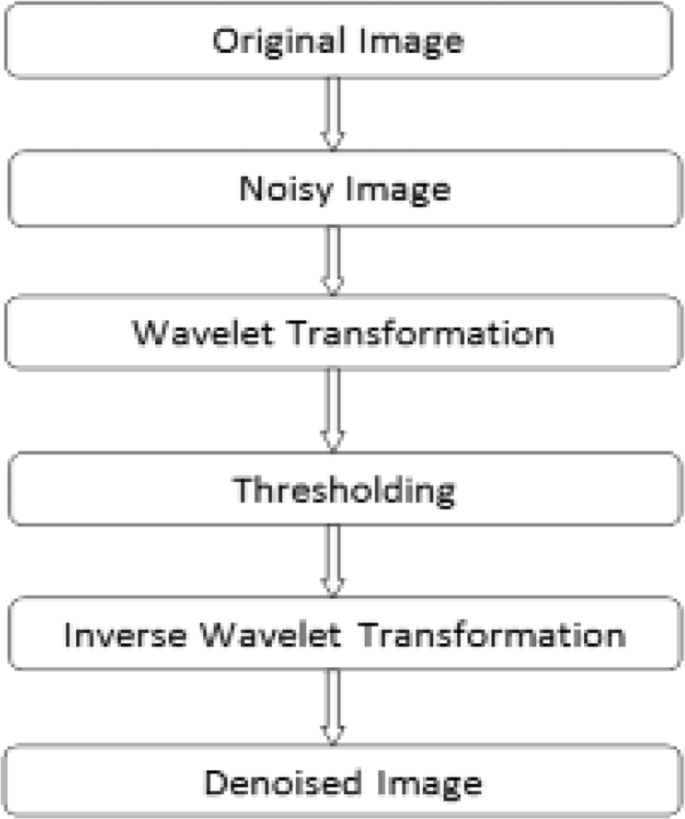
The basic framework of the wavelet transform based image denoising
-
The wavelet coefficients are denoised by using the wavelet thresholding technique.
-
The inverse discrete wavelet transform is applied to the modified coefficients to get the denoised image.

2.3.2.1 Wavelet thresholding approach for image denoising
Let the original image be {fij} of size M×N, where M, N is some integer power of 2. It has been corrupted by an additive zero-mean white and homogeneous Gaussian noise {nij}, with standard deviation σ, and one observes:
The goal is to estimate the denoised image {fij′} from noisy observation {gij}.
It is convenient to label the sub-bands of the transform as in Fig. 2. The sub-bands HHk, HLk, and LHk are called the details, where k is the level ranging from 1 to J, where J is the largest level. The sub-band LLJ is the low resolution residual. The wavelet transform is applied to (13) to obtain the wavelet coefficients cij. Then, the wavelet thresholding technique is used to filter each wavelet coefficient from the detail sub-bands with a threshold function to obtain the modified coefficients. Finally, the inverse wavelet transform is applied to the modified coefficients to get the denoised image. There are two thresholding methods frequently used. The soft-thresholding function (also called the shrinkage function):
takes the argument and shrinks it towards zero by the threshold T.
The other popular alternative is the hard-thresholding function:
which keeps the input if it is larger than the threshold; otherwise, it is set to zero. The wavelet thresholding procedure removes noise by thresholding only the wavelet coefficients of the detail sub-bands, while keeping the low-resolution coefficients unaltered [7, 30].
Donoho et al. [8] have discussed a simple, but influential wavelet-based denoising pattern known as VisuShrink. The outcomes of VisuShrink are stable along with an alluring visual feature. VisuShrink uses the universal threshold, T, which is proportional to the standard deviation of the noise, and it is defined as follows [9]:
where σ2 is the noise variance, defined as follows:
where cij∈HH1 sub-band thresholding.
S: Number of pixel for the test image.
2.3.3 Total variation denoising method
TV-based regularization is the most influential research in the field of image denoising. TV regularization is based on the statistical fact that natural images are locally smooth, and the pixel intensity gradually varies in most regions. It has achieved great success in image denoising because it cannot only effectively calculate the optimal solution but also retain sharp edges.
The l1 total variation functional was first introduced by Rudin, Osher, and Fatemi (ROF) [40] to address image-denoising problems. It is formulated as:
where \(\hat {f}\) is the reconstructed denoised image, f is the noisy image, ∥.∥1 is the l1-norm, ∥.∥2 is the l2-norm, and σ is an error tolerance included to account for noisy data. The choice of technique for solving l1 regularization-based problems is crucial, as l1 is nonlinear; therefore, the computational burden can increase significantly using classic gradient-based methods. The recently published Split Bregman (SB) method [27, 41] is a simple and efficient algorithm for solving l1 regularization-based problems that makes it possible to split the minimization of l1 and l2 functionals. By applying the SB method to image denoising proposed in [27], the authors showed that the TV-denoising problem solved using SB formulation was computationally efficient, given that the SB formulation leads to a problem that can be solved using Gauss–Seidel and Fourier transform methods.
2.3.4 BM3D denoising method
The BM3D method [28] is a famous denoising method. It has become a baseline algorithm to test the performance of denoising algorithms. BM3D includes the following steps: the first step is block matching: for each image block located at j, the similar image blocks with size \(\sqrt {n}\times \sqrt {n}\) are collected in groups with member number Ij. Image blocks in each group are stacked together to form a \(\sqrt {n}\times \sqrt {n}\times I_{j}\) 3D data array. Second, the sparsity regularization step, the 3D arrays are decorrelated by using an invertible sparse 3D transform such as discrete cosine transform (DCT) [42] and then are filtered by thresholding or Wiener filtering. Finally, the restoration is obtained by aggregating all the estimated image patches.
2.4 Proposed denoising method
Suppose the input noisy image y is from a clean image x contaminated by additive zero-mean white and homogenous Gaussian noise z, with standard deviation σ. The measured image y is, thus
We desire to design an algorithm that can remove the noise from y, getting a denoised image \(\hat {x}\) as close as possible to the original image x. As shown in Fig. 4, the proposed denoising method consists of three steps:
-
In the first step, discrete wavelet transform is applied to the noisy image y, to get the approximation and wavelet coefficients.
Fig. 4 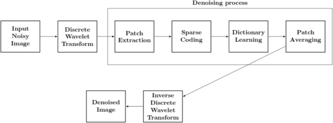
Block diagram of the proposed denoised method
-
In the second step, approximation and wavelet coefficients are denoised by using an adaptive dictionary learned on the set of extracted patches from wavelet representation of the noisy image, by the K-SVD as a dictionary learning algorithm.
-
In the third step, inverse discrete wavelet transform is applied for reconstructing the image, which results in the denoised image \(\hat {x}\).

The detailed steps of the proposed method can be given bellow:
In (19), we assume clear image x of size \(\sqrt {n}\times \sqrt {n}\) pixels and then use 2D discrete wavelet transform on the noisy image y. According to (19) and the property of wavelet transform, we have:
where Wy, Wx, and Wz are the wavelet transform of y, x, and z, respectively. Just like the K-SVD algorithm, learning dictionary on small image patches, note each small patch Wxij=RijWx of size \(\sqrt {n}\times \sqrt {n}\) in every location (i,j) of Wx. The matrix Rij is an n×N matrix that extracts the (ij) block size of n×1 pixels from the image Wx. For the image Wx of size \(\sqrt {n}\times \sqrt {n}\), the summation over i,j includes \((\sqrt {N}-\sqrt {n}+1)^{2}\) items, considering all image patches of size \(\sqrt {n}\times \sqrt {n}\) in Wx with overlaps. When redundant dictionary D∈Rn×k is given, according to the sparse prior of wavelet coefficients, every patch Wxij has a sparse representation with bounded error, we get:
The Lagrange form of it is:
By maximum a posteriori estimation, denoising of Wy is equivalent to the energy minimization problem:
In this expression, the first term is the log-likelihood between Wx and Wy, and λ depends on \(\parallel Wx-Wy \parallel _{2}^{2}\leq Cst\times \sigma ^{2} \). The second and the third terms are the sparse prior of wavelet coefficients.
When D is known, we can solve (23) by two steps. First, let Wx=Wy, thus (23) is equivalent to solve \((\sqrt {N}-\sqrt {n}+1)^{2}\) problems of (22) which can be solved by OMP. This step is called sparse coding. Second, when getting \(\hat {\alpha }_{ij}\) for all (ij) locations, fix them and turn to update Wx. Returning to (23), we need to solve:
This is a simple quadratic term that has a closed-form solution of the form:
This expression says the averaging of the denoised patches and is called patches averaging step. Given the updated, we can repeat the sparse coding stage, working on the already denoised patches. Once this is done, a new averaging should be calculated, and so on, and so forth. Finally, the satisfying \(\hat {\alpha }_{ij}\) and \(W\hat {x}\) are obtained. In practice, the dictionary D is unknown and we can get it by learning which is same to [23]. After fusion dictionary learning in (23), we get the denoising model as follows:
In this work, the K-SVD algorithm is used to learn and update the initial redundant DCT dictionary, and Wyij is the training set. As so far, we can solve (26) as follows: (a) Given the initial dictionary D and let Wx=Wy, then compute \(\hat {\alpha }_{ij}\) by (21); (b) update initial dictionary D to \(\hat {D}\) using K-SVD; and (c) compute \(W\hat {x}\) by (25). Finally, let \(\hat {D}\) and \(W\hat {x}\) are the initial D and Wx, then repeat the above process until getting the denoised image \(W\hat {x}\). As so far, we have finished the denoising process in the wavelet domain, the 2D inverse discrete wavelet transform is used to get the restoration image \(\hat {x}\). The following sequence defines our proposed algorithm:

3 Results and discussion
In this section, we aim to demonstrate the advantages and the performance that our proposed wavelet denoising approach based on unsupervised learning model has.
Our proposed algorithm is evaluated and compared with four representative and state-of-the-art denoising algorithms: the wavelet thresholding approach for image denoising, the sparse representation-based K-SVD denoising method in the image domain, the TV denoising method, and the BM3D denoising method.
In our experiments, we choose five well-known images as test images, including “Barbara,” “House,” “Flinstones,” “Bridge,” and “Fingerprint.” Each image is contaminated by adding zero-mean white Gaussian noise with various deviations. These following parameters are used in our proposed method: for the choice of the best wavelet basis, we test several wavelets under each noise level for all images and take the results with the highest PSNR for comparison, as a result, for the wavelet transform and inverse wavelet transform, we choose the Coiflet wavelet transform (MATLAB ’coif’) for the two images: “House,” “Fingerprint,” and Symlet wavelet transform (MATLAB ’sym’) for the rest of images, the size of patches n=64, the number of dictionary elements k=256, the Lagrange multiplier λ=30/σ, and the noise gain C=1.15.
Since we evaluate denoised images with the measures of the PSNR and SSIM index, the formulas of the PSNR and SSIM are also given. The PSNR is estimated based on the mean square error (MSE) as:
where I1 and I2 denotes two images of size N1×N2, I1(i,j) represents the pixel value on the ith row and jth column of I1. The SSIM index is defined as:
where \(\mu _{I_{1}}\) and \(\sigma _{I_{1}}\) denote the average gray values and the variance for I1, \(\sigma _{I_{1}I_{2}}\) represents the covariance between the two images I1 and I2, and the symbols C1 and C2 are two small constants [43]. The higher the value of PSNR or SSIM, the closer is the denoised image I2 to the original image I1, hence the more accurate is the denoising.
The comparison of quantitative results is shown in Tables 1 and 2. A visual comparison is shown in Figs. 5, 6, 7, 8, 9, 10, 11, 12, 13, 14, 15, and 16.

Denoising performance comparisons of “Barbara” with the noise deviation σ=10 by different methods. a Noisy image. b Denoised image by wavelet thresholding. c Denoised image by TV. d Denoised image by K-SVD. e Denoised image by BM3D. f Denoised image by the proposed method

Denoising performance comparisons of “House” with the noise deviation σ=10 by different methods. a Noisy image. b Denoised image by wavelet thresholding. c Denoised image by TV. d Denoised image by K-SVD. e Denoised image by BM3D. f Denoised image by the proposed method

Denoising performance comparisons of “Barbara” with the noise deviation σ=50 by different methods. a Noisy image. b Denoised image by wavelet thresholding. c Denoised image by TV. d Denoised image by K-SVD. e Denoised image by BM3D. f Denoised image by the proposed method

Denoising performance comparisons of “Barbara” with the noise deviation σ=70 by different methods. a Noisy image. b Denoised image by wavelet thresholding. c Denoised image by TV. d Denoised image by K-SVD. e Denoised image by BM3D. f Denoised image by the proposed method

Denoising performance comparisons of “House” with the noise deviation σ=50 by different methods. a Noisy image. b Denoised image by wavelet thresholding. c Denoised image by TV. d Denoised image by K-SVD. e Denoised image by BM3D. f Denoised image by the proposed method

Denoising performance comparisons of “House” with the noise deviation σ=70 by different methods. a Noisy image. b Denoised image by wavelet thresholding. c Denoised image by TV. d Denoised image by K-SVD. e Denoised image by BM3D. f Denoised image by the proposed method

Denoising performance comparisons of “Flinstones” with the noise deviation σ=10 by different methods. a Noisy image. b Denoised image by wavelet thresholding. c Denoised image by TV. d Denoised image by K-SVD. e Denoised image by BM3D. f Denoised image by the proposed method

Denoising performance comparisons of “Flinstones” with the noise deviation σ=70 by different methods. a Noisy image. b Denoised image by wavelet thresholding. c Denoised image by TV. d Denoised image by K-SVD. e Denoised image by BM3D. f Denoised image by the proposed method

Denoising performance comparisons of “Bridge” with the noise deviation σ=10 by different methods. a Noisy image. b Denoised image by wavelet thresholding. c Denoised image by TV. d Denoised image by K-SVD. e Denoised image by BM3D. f Denoised image by the proposed method

Denoising performance comparisons of “Bridge” with the noise deviation σ=70 by different methods. a Noisy image. b Denoised image by wavelet thresholding. c Denoised image by TV. d Denoised image by K-SVD. e Denoised image by BM3D. f Denoised image by the proposed method

Denoising performance comparisons of “Fingerprint” with the noise deviation σ=10 by different methods. a Noisy image. b Denoised image by wavelet thresholding. c Denoised image by TV. d Denoised image by K-SVD. e Denoised image by BM3D. f Denoised image by the proposed method

Denoising performance comparisons of “Fingerprint” with the noise deviation σ=70 by different methods. a Noisy image. b Denoised image by wavelet thresholding. c Denoised image by TV. d Denoised image by K-SVD. e Denoised image by BM3D. f Denoised image by the proposed method
Let’s first see the PSNR and SSIM results by different methods on the five test images. The statistical results of the five methods are given in the PSNR measure in Table 1. The results show that the proposed method outperforms the three denoising methods: wavelet thresholding, TV, and K-SVD, in all cases. Compared to the BM3D, for the two images: “Barbara” and “House”, the proposed method has the lowest PSNR value under some noise level variations, but for the rest of images, the proposed method has the higher PSNR measures than BM3D. The statistical results of the five methods are also recorded in the SSIM measure as shown in Table 2. Based on these results, we can deduce that our proposed method is always better than the other denoising methods, which assures the efficiency of our algorithm.
Let us then focus on the visual quality evaluation of these denoising algorithms. We take two example images: “Barbara” and “House”, to show that although BM3D has higher PSNR measures than the proposed method under some noise level variations for these two images, the proposed method has better visual quality than the BM3D method. To show the performance under different levels of noise, for the two images: “Barbara” and “House”, we show the results under low-level noise with standard deviation σ=10 and high-level noise with σ=50 and σ=70. For the rest of images, we show the denoising results with the noise deviation σ=10 and σ=70, by different methods. The Figs. 5, 6, 7, 8, 9, 10, 11, 12, 13, 14, 15, and 16 demonstrate the denoising results produced by the proposed method and the state-of-the-art denoising methods: wavelet thresholding, TV, K-SVD, and BM3D. The results show that under low-level noise with σ=10, the denoised images by the proposed method and the BM3D method are very similar in real visual perception, and they have much better visual quality than all the other methods. Under high noise levels, the results show that the edges are well preserved, the textures and more details are better restored, and least artifacts exist in the result of our proposed method. The performance of the wavelet thresholding approach, the K-SVD, and the TV denoising method is the worst in various noise levels; it is easy to see that the restored images contain too many artifacts, the image edges and flat areas are blurred, and a number of details and textures are lost. It also found in the experiments that the proposed method has much better visual quality than the BM3D method that produces too many artificial ringing effects which are caused by stacking the image blocks and erroneous grouping.
Depending on the size of the image, the execution of the main proposed algorithm requires an average of 17 s to 2 min on Intel(R) Core(TM) i3-2330M CPU 2.20 GHz computer. The average time required by the other algorithms to complete their executions is given as follows: the wavelet thresholding approach for image denoising: 2 to 5 s, the sparse representation-based K-SVD denoising method in the image domain: 15 s to 2 min, the TV denoising method: 12 to 30 s, and the BM3D denoising method: 5 to 15 s. The proposed algorithm is slower than the other denoising methods, due to the use of the K-SVD as a dictionary learning algorithm that needs many iteration steps.
Our proposed method performs better than the state-of-the-art denoising methods, due to the merits of the wavelet transform and to the use of an adaptive dictionary devoted to noise reduction instead of using the thresholding operator.
4 Conclusion
We propose in this work a new method for image denoising. The approach taken aims at exploiting the merits of the wavelet transform: sparsity, multi-resolution structure, similarity with the human visual system, and good localization properties both in space and frequency, to adapt an unsupervised dictionary learning algorithm for creating a dictionary devoted to eliminate the useless information while keeping most significant ones. Experiments illustrate that the proposed method achieves a better performance than some other well-developed denoising methods, especially in PSNR, SSIM index, and visual effects. In future work, we will be focused more on reducing the computational cost of the proposed model.
Availability of data and materials
The benchmark used to demonstrate the effectiveness of the proposed approach is composed of five standard images used for image processing. These images are frequently found in literature.
Abbreviations
- K-SVD:
-
K-singular value decomposition
- PSNR:
-
Peak signal-to-noise ratio
- SSIM:
-
Structural similarity
- WT:
-
Wavelet transform
- TV:
-
Total variation
- BM3D:
-
Block-matching and 3D filtering
- MRA:
-
Multi-resolution analysis
- DWT:
-
Discrete wavelet transform
- OMP:
-
Orthogonal matching pursuit
- SVD:
-
Singular value decomposition
- ROF:
-
Rudin, Osher, and Fatemi
- SB:
-
Split Bregman
- DCT:
-
Discrete cosine transform
- MSE:
-
Mean squared error
References
R. Kenneth, Digital Image Processing (Prentice Hall, New Jersey, 1979).
A. K. Boyat, B. K. Joshi, A review paper: noise models in digital image processing. Signal Image Process. Int. J. (SIPIJ). 6(2), 63–75 (2015).
M. Diwakar, M. Kumar, A review on CT image noise and its denoising. BioMed. Signal Process. Control. 42:, 73–88 (2018).
L. Fan, F. Zhang, H. Fan, et al., Brief review of image denoising techniques. Vis. Comput. Ind. Biomed. Art. 2(7), 1–12 (2019).
S. Mallat, A wavelet tour of signal processing: the sparse way 3rd edition (Academic Press, Elsevier, Burlington, 2008).
J. N. Ellinas, T. Mandadelis, A. Tzortzis, et al., Image de-noising using wavelets. T.E.I Piraeus Appl. Res. Rev.IX(1), 97–109 (2004).
S. Grace Chang, B. Yu, M. Vattereli, Adaptive wavelet thresholding for image denoising and compression. IEEE Trans. Image Process. 9:, 1532–1546 (2000).
D. L. Donoho, I. M. Johnstone, Adapting to unknown smoothness via wavelet shrinkage. J. Am. Stat. Assoc.90(432), 24–1200 (1995).
D. L. Donoho, De-noising by soft-thresholding. IEEE Trans. Inf. Theory. 41(3), 613–627 (1995).
D. Gupta, M. Ahmad, Brain MR image denoising based on wavelet transform. Int. J. Appl. Technol. Eng. Explor.5(38), 11–16 (2018).
V. Fedak, A. Nakonechnyy, in Technical Transaction on Electrical Engineering. Adaptive wavelet thresholding for image denoising using SURE Minimization and Clustering of Wavelet Coefficients, (2015), pp. 197–210.
M. K. Mıhcak, I. Kozintsev, K. Ramchandran, P Moulin, Low-complexity image denoising based on statistical modeling of wavelet coefficients. IEEE Signal Process. Lett.6(12), 300–303 (1999).
S. G. Chang, B. Yu, M. Vetterli, Spatially adaptive wavelet thresholding with context modeling for image denoising. IEEE Trans. Image Process.9(9), 1522–1531 (2000).
A. Pizurica, W. Philips, I. Lamachieu, et al., A joint inter and intrascale statistical model for Bayesian wavelet based image denoising. IEEE Trans. Image Process.11(5), 545–557 (2002).
D. Donoho, Wedgelets: nearly minimax estimation of edges. Ann. Stat.27(3), 859–897 (1999).
E. Candes, D. L. Donoho, Recovering edges in ill-posed inverse problems: optimality of curvelet frames. Ann. Stat.30(3), 784–842 (2002).
E. Candes, D. L. Donoho, New tight frames of curvelets and the problem of approximating piecewise C2 image with piecewise C2 edges. Commun. Pure Appl. Math.57:, 219–266 (2003).
E. Pennec, S. Mallat, Sparse geometric image representations with bandelets. IEEE Trans. Image Process.14(4), 423–438 (2005).
S. Mallat, E. L. Pennec, Bandelet image approximation and compression. SIAM Multiscale Model. Simul.4(3), 992–1039 (2005).
M. Do, M. Vetterli, Frame pyramids. IEEE Trans. Signal Process. 51(9), 2329–2342 (2003).
S. Mallat, G. Peyre, Orthogonal bandlet bases for geometric images approximation. Coomun. Pure Appl. Math.61(9), 1173–1212 (2008).
W. T. Freeman, E. H. Adelson, The design and the use of steerable filters. IEEE Trans. Pattern Anal. Mach. Intell.13(9), 891–906 (1991).
M. Aharon, M. Elad, A. M. Bruckstein, The K-SVD: an algorithm for designing of overcomplete dictionaries for sparse representation. IEEE Trans. Signal Process.54(11), 4311–4322 (2006).
M. Elad, M. Aharon, Image denoising via sparse and redundant representations over learned dictionaries. IEEE Trans. Image Process.15(12), 3736–3745 (2006).
M. Elad, M. Aharon, Image denoising via learned dictionaries and sparse representation. CVPR. 1:, 895–900 (2006).
MH. Alkinani, MR. El-Sakka, Patch-based models and algorithms for image denoising: a comparative review between patch-based images denoising methods for additive noise reduction. EURASIP J. Image Video Process.58:, 1–27 (2017).
T. Goldstein, S. Osher, The split Bregman method for l1 regularized problems. SIAM J. Imaging Sci.2(2), 323–343 (2009).
K. Dabov, A. Foi, V. Katkovnik, K. Egiazarian, Image denoising by sparse 3D transform-domain collaborative filtering. IEEE Trans. Image Process.16(8), 2080–2095 (2007).
S. Mallat, A theory for multiresolution signal decomposition: the wavelet representation. IEEE Transaction on Pattern Analysis and Machine Intelligence. 12(7), 674–693 (1980).
S. Kother Mohideen, S. Arumuga Perumal, M. Mohamed Sathik, Image de-noising using discrete wavelet transform. IJCSNS Int. J. Comput. Sci. Netw. Secur.8(1), 213–216 (2008).
M. Antonini, M. Barlaud, P. Mathieu, et al., Image coding using wavelet transform. IEEE Trans. Image Process.1(2), 205–220 (1992).
H. Demirel, G. Anbarjafari, Discrete wavelet transform-based satellite image resolution enhancement. IEEE Trans. Geosci. Remote. Sens.49(6), 1997–2004 (2011).
G. Fan, X. G. Xia, Wavelet-based texture analysis and synthesis using hidden Markov models. IEEE Trans. Circ. Syst. I Fundam. Theory Appl.50(1), 106–120 (2003).
D. R. Nayak, R. Dash, B. Majhi, Brain MR image classification using two-dimensional discrete wavelet transform and AdaBoost with random forests. Neurocomputing. 177:, 188–197 (2016).
M. Misiti, Y. Misiti, G. Oppenheim, M. JPoggi, Wavelet ToolboxTM 4 User’s Guide (The MathWork Inc., MA, 2009).
D. J. Field, ed. by D. M. Farge, R. Hunt, and J. C. Vassilicos. Wavelets, fractals and Fourier transform (Clarendon PressOxford, 1993).
Y. C. Pati, R. Rezaiifar, P. S. Krishnaprasad, Orthogonal matching pursuit: recursive function approximation with applications towavelet decomposition. 27th Annu. Asilomar Conf. Signal Syst. Comput.43(1), 40–44 (1993).
D. L. Donoho, M. Elad, V. Temlyakov, Stable recovery of sparse overcomplete representations in the presence of noise. IEEE Trans. Inf. Theory. 52(1), 6–18 (2006).
J. A. Tropp, Just relax: convex programming methods for subset selection and sparse approximation. IEEE Trans. Inf. Theory. 51(3), 1030–1051 (2005).
L. I. Rudin, S. Osher, E. Fatemi, Nonlinear total variation based noise removal algorithms. Phys. D.60(1), 259–268 (1992).
J. Chamorro-Servent, J. F. Abascal, J. Aguirre, et al., Use of split Bregman denoising for iterative reconstruction in fluorescence diffuse optical tomography. J Biomed. Opt.18(7), 076016 (2013).
N. Ahmed, T. Natarajan, K. R. Rao, Discrete cosine transform. IEEE Trans. Comput.23(1), 90–93 (1974).
Z Wang, A. C Bovik, H. R Sheikh, et al., Image quality assessment: from error visibility to structural similarity. IEEE Trans. Image Process.13(4), 600–612 (2004).
Acknowledgements
Not applicable.
Funding
Not applicable.
Author information
Authors and Affiliations
Contributions
Authors’ contributions
All authors contributed equally in this work. The authors read and approved the final manuscript.
Authors’ information
Khawla Bnou, first author, is a PhD student of the Laboratory of Applied Mathematics and Computer Science, Faculty of Science and Techniques, Cadi Ayyad University, Marrakesh, Morocco. Said Raghay, PhD, Laboratory of Applied Mathematics and Computer Science, Faculty of Science and Techniques, Cadi Ayyad University, Marrakesh, Morocco. Abdelilah Hakim, PhD, Laboratory of Applied Mathematics and Computer Science, Faculty of Science and Techniques, Cadi Ayyad University, Marrakesh, Morocco.
Corresponding author
Ethics declarations
Competing interests
The authors declare that they have no competing interests.
Additional information
Publisher’s Note
Springer Nature remains neutral with regard to jurisdictional claims in published maps and institutional affiliations.
Rights and permissions
Open Access This article is licensed under a Creative Commons Attribution 4.0 International License, which permits use, sharing, adaptation, distribution and reproduction in any medium or format, as long as you give appropriate credit to the original author(s) and the source, provide a link to the Creative Commons licence, and indicate if changes were made. The images or other third party material in this article are included in the article’s Creative Commons licence, unless indicated otherwise in a credit line to the material. If material is not included in the article’s Creative Commons licence and your intended use is not permitted by statutory regulation or exceeds the permitted use, you will need to obtain permission directly from the copyright holder. To view a copy of this licence, visit http://creativecommons.org/licenses/by/4.0/.
About this article

Cite this article
Bnou, K., Raghay, S. & Hakim, A. A wavelet denoising approach based on unsupervised learning model. EURASIP J. Adv. Signal Process. 2020, 36 (2020). https://doi.org/10.1186/s13634-020-00693-4
Received:
Accepted:
Published:
DOI: https://doi.org/10.1186/s13634-020-00693-4