- Research
- Open access
- Published:
3D shape representation with spatial probabilistic distribution of intrinsic shape keypoints
EURASIP Journal on Advances in Signal Processing volume 2017, Article number: 52 (2017)
Abstract
The accelerated advancement in modeling, digitizing, and visualizing techniques for 3D shapes has led to an increasing amount of 3D models creation and usage, thanks to the 3D sensors which are readily available and easy to utilize. As a result, determining the similarity between 3D shapes has become consequential and is a fundamental task in shape-based recognition, retrieval, clustering, and classification. Several decades of research in Content-Based Information Retrieval (CBIR) has resulted in diverse techniques for 2D and 3D shape or object classification/retrieval and many benchmark data sets. In this article, a novel technique for 3D shape representation and object classification has been proposed based on analyses of spatial, geometric distributions of 3D keypoints. These distributions capture the intrinsic geometric structure of 3D objects. The result of the approach is a probability distribution function (PDF) produced from spatial disposition of 3D keypoints, keypoints which are stable on object surface and invariant to pose changes. Each class/instance of an object can be uniquely represented by a PDF. This shape representation is robust yet with a simple idea, easy to implement but fast enough to compute. Both Euclidean and topological space on object’s surface are considered to build the PDFs. Topology-based geodesic distances between keypoints exploit the non-planar surface properties of the object. The performance of the novel shape signature is tested with object classification accuracy. The classification efficacy of the new shape analysis method is evaluated on a new dataset acquired with a Time-of-Flight camera, and also, a comparative evaluation on a standard benchmark dataset with state-of-the-art methods is performed. Experimental results demonstrate superior classification performance of the new approach on RGB-D dataset and depth data.
1 Introduction
There has been an explosive growth in the usage of 3D models in recent years due to quantum jump in 3D sensing technology to model, digitize, and visualize 3D shapes. This digital revolution can be attributed to substantial and continuous improvements in microelectronics, microoptics, and microtechnology. These expensive 3D sensors which were once only available for specialized industrial applications are now commercially available for research communities and general public for 3D reconstruction, mapping, SLAM, human-machine interaction, service robotics, gaming, preserving cultural heritage, security and surveillance, 3D printing, CAD, and others [1]. As a direct result of this, there has been an exponential increase in the amount of 3D models usage and wherefore determining the similarity between 3D models has become crucial and is also at the core of shape-based object detection, recognition, and classification. In order to compare similarity between two shapes, a suitable numerical representation of the shapes is necessary to output a quantitative similarity score. A shape descriptor is numerical representation of a 2D or 3D shape in the form of vectors or graph data-structures and is extensively used to extract and describe features at visually important regions in the object. The distance between two feature vectors quantitatively represents the dissimilarity between their corresponding shapes; the more similar the objects are, the lower the dissimilarity score, and a score of zero indicates that the two shapes are identical [2]. The dissimilarity measure can be formalized by a function defined on pairs of descriptors indicating the degree of their resemblance; a dissimilarity measure d on a set S is a non-negative valued function \({d}:{S}\times {S}\mapsto \mathbb {R}^{+}\cup \{0\}\). In general, dissimilarity score follows the properties of identity, positivity, symmetry, triangle inequality, and transformation invariance [3]. Many decades of active research has been done on shape representation for object classification, recognition, and detection. As a result, many different approaches have been proposed to solve this problem, and many taxonomical classifications of the basic idea behind these approaches exist. An elementary classification can be based on application to 2D or 3D shapes (see Fig. 1). In existing literature, 2D shape descriptors are classified into two categories: contour-based, region-based, and a hybrid of these two [4–6]. A very good generic classification of shape-feature extraction approaches is given by Yang et al. [7]. And for matching 2D shapes involving non-rigid deformations, the methods involve finding intrinsic near isometries [8–10] or perform shape matching in appropriate quotient space, where the symmetry has been identified and factored out [11]. The 3D descriptors, on the other hand, exclusively depends on the object’s surface properties or its interior rather than attributes like color and texture [12] which are, otherwise, extensively used in 2D image recognition and retrieval [13]. The development of a good 3D shape descriptor poses several technical challenges, including, in particular, the high data complexity of 3D models [14–16] and their representations involving dynamism, shape flexibility and structural variations [14, 16, 17], noise, occlusions, and incompleteness present in them [12, 18]. Zhang et al. [13], Tangelder et al. [19], Akgül et al. [20], and Kazmi et al. [4] have broadly classified the 3D shape descriptor approaches into three classes: feature-based, graph-based, and others. Others are either geometry-based, 2D view-based, or transform-based methods.
-
1.
Fig. 1 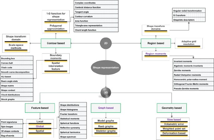
Taxonomical classification of shape analysis techniques. At the root, they can be classified based on dimensionality of the model (2D or 3D). The proposed approach is a combination of region, feature, and graph-based method as highlighted with indigo font color
- 2.
- 3.

Feature-based methods have gained prominence as a consequence of SIFT invention by Lowe [39]. Since then, they have become de facto standard in image processing due to their good performance. The term features is often used to refer to persistent elements in an image [26]. Zhang et al. [13] have classified feature-based approaches into four types:
-
1.
Local features;
-
2.
Global features;
-
3.
Distribution-based;
-
4.
Spatial map.
Local features extract information around salient regions (visually important) in the image, while global features describe the whole image. This local or global “description” of the image is called feature descriptors or just descriptors. A shape descriptor is a numerical representation of a 2D or 3D shape in the form of vectors or graph data-structures. Graph-based shape analysis is essentially different from vector-based feature descriptors: they encode the geometrical and topological shape properties in a more faithful manner than vector-based descriptors, however, at the expense of their complexity and difficulty to construct. Multi-resolution Reeb graphs [29] and skeletal graphs [30] are the classic examples of this type. On the contrary, geometry-based methods either consider multiple views of the model or exploit the geometric and spatial properties of the points and weigh them. In general, they can be further classified into the following types [19]:
-
View-based. A descriptor of each 3D model is constructed from multiple orthographic view directions. Similarity search is done with either shock graph matching [40, 41] or light-field descriptor dissimilarity [31].
-
Deformation-based. A pair of 2D/3D shapes is compared by measuring the amount of deformation required to register the shapes exactly. However, Shape fitting [42] or Shape evolution [43] are difficult for 3D shapes.
-
Point set methods. Here, the descriptor of a shape is given by weighted 3D points. In the first step, the shape is decomposed into its components, and then each component is represented using a weighted point [37]. Curvature of points for example can be a very good measure for weighing [38].
-
Volumetric error. It is based on calculating a volumetric error between one object and a sequence of offset hulls of the other object [34]. Sánchez-Cruz and Bribiesca [33] presented a method which relates the volumetric error between two voxelized shapes to a transportation distance measuring how many voxels have to move, and how far, to change one shape into another.
Shape analysis approaches can also be flattened into two groups: heat diffusion [15, 17, 44, 45] and non-diffusion-based [21, 24, 46] shape features, according to [47].
The proposed approach in this article can be distantly related to Osada’s shape distributions method [21]. Shape distribution is a feature-based idea which is a combination of global and distribution-based methods. It is a simplistic method which reduces the shape matching problem to sampling, normalizations, and comparison of probability distributions. It represents the shape signature for a 3D model as a probability distribution sampled from a shape function measuring geometric properties of the 3D model. This generalization of geometric histograms is called shape distribution (Fig. 2). Shape distributions measure geometric properties relied on distance, angle, area, and volume measurements between random surface points. Osada et al. [21] have experimented five shape functions (Fig. 3):
-
A3: angle formed by three random surface points,
Fig. 2 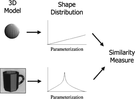
Shape distribution-based similarity measurement [21]. The 3D models are represented as distribution of Euclidean shape functions and similarity is measured using histogram-based fidelity scores
Fig. 3 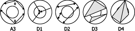
Shape functions by Osada et al. [21]. All the distances are calculated on Euclidean space
-
D1: distance of a surface point to the center of mass of the model,
-
D2: distance between two random surface points,
-
D3: square root of the area of the triangle defined by three random points,
-
D4: cube root of the volume of the tetrahedron defined by four surface points,


which were chosen for their simplicity to compute and understand, and also because they produce distributions that are invariant to rigid motions and tessellation, insensitive to small perturbation and scale invariant (in case of A3).
However, sensor data is actually 2.5D, and it can only give the partial view information of an object in single acquisition. In order to recognize the object in any pose in real world, it is necessary to have a complete 3D information of the object or multiple complementary views of the same object. As a result, the shape of an object cannot be determined by a single view, and shape distribution for the same object is completely different when viewed from another pose. Interestingly, the 3D keypoints are repeatable and consistent across different views. This wonderful property of 3D keypoints has been realized, the same five shape functions by Osada et al. [21] are analyzed, and it has been found that the geometric distributions of 3D keypoints are unique for individual object. Good 3D keypoints are like anchor points which are stable and holds the object for any rigid deformation/transformation. The shape distribution of them are similar across multiple views, and when trained using machine, learning algorithms can efficiently classify the object’s instances or categories. In previous work, performance evaluation of different 3D keypoint detectors was conducted on RGB-D and depth data [48], and it has been observed that ISS3D and SIFT3D are most repeatable keypoints and robust. In this article, the PDFs of geometric/spatial distribution of ISS3D keypoints has been analyzed and successfully exploited to represent an object. Euclidean and topological space-based norms are considered to build these distributions. KPD (KeyPoint Distribution) term is used to refer the distributions that are based on Euclidean norms and GKPD (Geodesic KeyPoint Distribution) is based on shortest paths on object’s manifold.
GKPD is a combination of feature, graph, and geometry-based methods. It capitalizes the pose invariance and stability of feature detectors. With graph representation of 3D points as nodes and geodesics between them as edges, the GKPD exploits the surface and topological information on the object’s manifold. And lastly, it considers the multiple complementary 2.5D views of the object to be able to detect it in the real world in any pose (a combination of view-based and point set methods in geometry-based approaches).
Detecting objects and labelling the real world scene with semantics (semantic mapping) are a must for future service robots equipped with 3D sensors like Time-of-Flight (ToF) cameras. The authors’ major contribution in this paper is threefold. First, to build a robust yet simple shape signature which considers the topography of an object and is consistent all through pose variations while being easy to implement. Second, to create a dataset of objects using a SwissRanger ToF camera [49] and an electronic device to measure pose changes. Third, to make a Machine Learning Model which learns these shape signatures and classifies the object instances or categories. The performance of KPD and GKPD is also compared with other state-of-the-art methods, utilizing the same Washington RGB-D dataset [50]. The pipeline of the complete methodology is shown in Fig. 4. The structure of the paper follows as a brief introduction to the importance of 3D shape analysis and different methods to represent shapes in Section 1. In the same section, a taxonomical classification of shape representation approaches and background for shape distribution is given. Related work is discussed in Section 2. In Section 3, an explanation of the need for a novel shape distribution signature is presented and definitions of some important concepts used are given. In Section 4, the description of the approach is presented with many subsections for the best understanding. Section 5 introduces few fundamental concepts about Machine Learning and two different standard libraries used. In Section 6, the utilized datasets are briefly described. In the last sections (Sections 7 and 8), experimental results and conclusions are presented.

Pipeline of the approach depicting different steps in it. The raw point cloud is filtered to make it noise-free. The filtered point cloud is then converted into a graphical representation, where every node is connected with every other node within certain sphere around it. Geodesics and L2 norms are calculated using Dijkstra algorithm. A distribution is made for each view of the object based on these distances and normalized to a PDF. In the last stage, these PDFs are fed into a classifier to build a hypothesis model
2 Related work
Since the introduction of Osada’s shape functions, there were many improvements done and also new shape functions have been implemented, whereas the authors of [51] proposed D2a, an improvement of D2 by considering area ratio of surfaces as additional dimension, whose of [52] split the D2 into three types of distances based on the geometric properties of the line connecting two points (IN, OUT, and MIXED) depending if the line lies completely inside the model or outside or both. They applied this method to compare solid CAD models. They also extended this method to automatically categorize a large model database [53]. A 3D histogram is implemented in [54]: two dimensions are for local and global shape signature and the third one is for distance between local shape pairs. This is known as Generalized Shape Distributions. Some shape histogram methods accumulate the surface points in the bins [22], while density-based employ richer sets of multivariate shape features with a kernel strategy to estimate the distribution [20, 55]. Ohbuchi et al. [56] investigate shape histograms that are discretely parametrized along the principal axes of inertia of the model and also extended D2 shape function by considering the angle between the surfaces on which two random points are located [57]. This extension called as Absolute Angle-Distance histogram (AAD) outperformed the D2 shape function but at the cost of computation time. Ohbuchi et al. further improved this method by multi-resolution approach, computing a number of alpha-shapes at different scales and computing AAD descriptor for each alpha-shape. Liu et al. [58] proposed another variation of shape distribution function (thickness histogram) estimating thickness of the 3D model from all directions. Rea et al. [59] described a surface portioning spectrum distribution, which measures the number of connected regions against a range of tolerance values [59]. In [60], they designed a shape descriptor based on the similarity between two 3D models by measuring the similarity of a series of 2D slices. They compared the similarity between two 2D slices using a D2 shape function [19]. The proposed approach uses Euclidean norm as well as geodesics, and it can be most closely related to the work of [21, 61–63] in that the authors also use probability distribution of geodesic distances as shape signature. However, it significantly differs from the geodesics extracted, the PDFs constructed, and the similarity measure considered in order to compare shapes and the concerned 2D/3D models themselves. A very good shape signature φ(Ω) ought to be invariant to certain class \(\mathcal {R}\) of deformations, φ(RΩ)=φ(Ω) for any \({R} \in \mathcal {R}\). Rabin et al. [61] considered for each point x∈S⊂Ω, the set \({\left \lbrace {d_{\varOmega }}({x}, {y})\right \rbrace }_{y \in {E} \subset \varOmega } \subset \mathbb {R^{+}}\) of distances to a subset of E⊂Ω. The set S is a discrete uniform sub-sampling of the manifold Ω obtained using farthest sampling principle [64] (e.g., red, green, and blue points in Fig. 5). The set E is equal to all points in manifold (E= Ω) for 3D surfaces and boundary points (E=∂Ω) for 2D shapes. At each location x∈S, the local geodesic descriptor \({p_{x}} \in \mathbb {R}^{d}\) is a vector of d quantiles,

Histogram of the distribution of the geodesic distance to several points [61]. The geodesics from seeds indicated by blue, green, and red propagate to all the points in the image, and their individual histogram distribution is depicted on the right
where ∀x∈S
is statistical quantile measure, 0≤α l ≤1 are equi-spaced values, and F x is cumulative distribution function of the set {d Ω(x,y),y∈E}. The global descriptor is then defined as a uniform sampling of local descriptors of n points on the manifold,
Then, Wasserstein metric related to the Monge Kantorovich optimal transport problem was used as similarity measure to compare φ(Ω) of different shapes. On the other hand, Ion et al. [63] considered geodesic eccentricity, i.e., quantile Q x (1), to construct a histogram-based descriptor, which actually calculates maximum geodesic distances corresponding to boundary points.
Hamza and Krim [62] calculated the geodesics on triangular meshes and constructed geodesic shape distributions which are then compared using Jensen-Shannon divergence [65]. They calculated the geodesic distance from the centroid of each triangle to all the centroids in the mesh and integrated it to get a global measure, \({f}: {C} \subset \mathbb {M} \rightarrow \mathbb {R}\),
where d c j is the area of the triangle having centroid c j and |C| is the total area of the manifold \(\mathbb {M}\).
Gal et al. [66] proposed pose-oblivious shape signature, a 2D histogram which is a combination of two scalar functions defined on the boundary surface of the 3D shape: local-diameter measures the diameter of the 3D shape in the neighborhood of each shape and centricity, which is similar to D2, considers average geodesic distance instead of Euclidean distance. Osada et al. [21] defined five shape functions which basically calculate Euclidean distances between the random points. They used their distributions to retrieve similar shapes, thanks to a couple of statistical dissimilarity measures.
All these approaches are applied to synthetic datasets (Table 1), where 3D models or 2D shapes are manually designed, hence, perfectly extracted, and do not represent real world scenarios. Consequently, all the above mentioned approaches fail in performance due to the second problem mentioned in Section 3.
3 Background
Shape distribution by Osada et al. [21] is a global feature-based approach which utilize shape functions developed on distance, angle, area, and volumetric measurements between random points on the 3D model. Osada et al. achieved very good classification results on the dataset from 3D polygonal models and developed a web-based search engine. However, shape distributions have some shortcomings. The shape functions are built on L 2 norms, in Euclidean space, without considering the topological information. As a result, two 3D models with different surfaces have similar distributions (see Fig. 6).

Similar D2 shape distributions for Swiss cheese and Gupta Socket [52]
The second problem arises from the fact that the sensor data is 2.5D, and it can only give the partial information of an object in single acquisition. As a result, the shape of an object cannot be determined from shape distribution from a single view, as shape distribution for the same object is completely different from those obtained from different views (Fig. 7). Apart from these two flaws, shape distribution is one of the basic methods to represent shape. In this paper, a novel idea is suggested to represent the shape of an object so as to recognize it in the real world in any pose. Those two shortcomings mentioned are overcome by considering the object manifold and efficient 3D keypoint detectors. The presented approach is completely different from Osada’s except the use of PDFs to represent shape.

D2 shape distribution for two different guitar poses (captured using ToF camera). Left: b is rotated 30° from a. Right: top represents a, bottom for b. The red points are actual D2 distribution of the views, and fitted with smoothing splines and polynomial curves (blue curves) of degree 9 instead of piecewise linear functions used by Osada et al. [21]
3.1 Minimal paths
The first problem is solved using geodesics or minimal paths instead of Euclidean distances; this preserves the topological information of the object. The geodesic distance d Ω(x s ,x e ) between two points x s , x e is the length of the geodesic curve γ ∗ on a Riemannian manifold \(\Omega \subset \mathbb {R}^{2}\) associated to the surface \({S} \subset \mathbb {R}^{3}\) [67]:
The length of the curve \(\bar {\gamma }\):
where T x is a tensor field (Riemannian metric) being positive definite matrix \({T}_{x} \in \mathbb {R}^{d\times d}\) and P(x s ,x e ) is a fixed pair of start (x s ) and end point (x e ):
Geodesics are easy to calculate on triangulated meshes and on 2D images. However, point clouds are often noisy and the data depend on physical properties like reflection and absorption of light by the objects (Fig. 8). As a result, unconnected sets of point clouds for the same object are frequently obtained. Triangulation of these kinds of point clouds often leads to unconnected meshes, on which calculating geodesics is not trivial. In this scenario, graph theory comes to rescue. Generally, the word “geodesic” is mostly used for surfaces and meshes; however, it is also commonly used for calculating the shortest paths on graphs. The numerical computation of geodesic distances has several applications including surface and shape processing, particularly segmentation [68, 69], sampling, meshing [70], and shape comparison [62, 63].

The four possible intrinsic reference frames as proposed and developed by [75]
3.2 3D keypoints
The second flaw, shape variation due to pose changes, can be tackled by considering efficient 3D keypoint detectors. The 3D keypoints or interest points are stable, repeatable, and consistent across different views. Good 3D points are like anchor points which are stable and hold the shape of the object for any rigid deformation or transformation [48]. Constructing shape functions on 3D keypoints instead of all the points on the surface seems a good bet.
4 Approach
There are four stages in the proposed approach (see Fig. 4). Firstly, the point cloud is pre-processed to obtain noise-free object representation and then detect ISS3D keypoints for every single view of all the objects. Then, each view of the object is transformed into a graph and the shortest paths between keypoints are calculated. Every view is then represented as probability distributions of geodesics. In the last stage, distribution learning and classification are carried out.
4.1 Point cloud filtering
The first step in the approach is to filter the point cloud from systematic and non-systematic noise. This has been achieved by using statistical outlier filters and jump edge filters [71]. The noise-free point cloud is then utilized in the next steps to construct graphs and distributions.
4.2 Intrinsic shape signatures
A meticulous experiment is conducted to determine the most stable and robust 3D keypoints for Washington RGB-D [50] data set and ToF dataset (Fig. 8). ToF dataset is a collection of several household objects (Fig. 17) obtained using a SwissRanger camera mounted on a Cartesian robot (AFMA) (Fig. 9 a, b). The absolute and relative repeatability tests [72, 73] of several 3D keypoint detectors are calculated using the pose information obtained from ICP [74] (augmented with AFMA pose estimates and Washington pose files). It has been discovered that intrinsic shape signatures, called here ISS3D, are more robust against rigid deformations than other detectors (see Fig. 10).

a, b AFMA robot’s effector mounted with SR-4K camera and focussed on the object

a Absolute repeatability and b relative repeatability w.r.t. threshold ε (in m) for different 3D keypoint detectors for Washington RGBD-D dataset and our depth data. A keypoint extracted from model M h , \({k^{i}_{h}}\) and transformed according to the ground-truth rotation and translation, (R hl , t hl ) is said to be repeatable if the distance from its nearest neighbor, \({k^{j}_{l}}\), in the set of keypoints extracted from the scene S l is less than threshold ε
Indeed, the intrinsic shape signature proposed by [75] characterizes the local/semi-local region of a point cloud, consisting of an intrinsic reference frame and a highly discriminative feature vector encoding the 3D shape characteristics. It uses a view-independent representation of the 3D shape to match shape patches from different views directly and a view-dependent transform encoding the viewing geometry to facilitate fast pose estimation. The ISS3D, S i ={F i ,f i } at a basis point p i , consists of two components. First, \({F_{i}=\left \{p_{i},\left \{e^{x}_{i},e^{y}_{i},e^{z}_{i}\right \}\right \}}\), an intrinsic reference frame with p i as origin and \({\left \{e^{x}_{i},e^{y}_{i},e^{z}_{i}\right \}}\) as set of basis vectors. Second, a 3D shape-feature vector, f i =(f i0,f i1,…,f i K−1), a view independent representation of the local/semi-local 3D shape. However, the basis specifies the vector of its axes in the sensor coordinate system, hence view dependent, and directly encodes the pose transform between the sensor coordinate system and the local object-oriented intrinsic frame. The first component, intrinsic reference frame F i at basis point p i with a supporting radius r frame , is defined using the eigen analysis of the point scatter matrix as follows:
-
1.
In the first step, each point p i is weighted with a value inversely proportional to the number of points in its spherical neighborhood of radius r density .
$$ {w_{i}}= \frac{1}{\left\|\left\{{p_{j}}:\left|{p_{j}}-{p_{i}}\right|<{r_{density}}\right\}\right\|} $$(8)This criterion actually helps for uniform weighing of the points, as some points are sparsely distributed.
-
2.
A weighted scatter or covariance matrix for p i using all its neighbors p j within a distance r frame is calculated:
$$ {COV(p_{i})}=\frac{\sum_{\left|p_{j}-p_{i}\right|<r_{frame}}{w_{j}}\left({p_{j}}-{p_{i}}\right)\left({p_{j}}-{p_{i}}\right)^{\intercal}}{\sum_{\left|p_{j}-p_{i}\right|<r_{frame}} {w_{j}}} $$(9) -
3.
The eigen values and eigen vectors are computed in the decreasing order of magnitude.
-
4.
A 3D coordinate system is constructed using p i as the origin, and e 1, e 2, and their cross product e 1 ⊗ e 2 as the x−, y−, and z− axes respectively. This reference system is actually the intrinsic coordinate system, F i , which is a characteristic of the local object shape and indifferent to viewpoint. However, the basis specifies the vector of its axes in the sensor coordinate system, hence view dependent, and directly encodes the pose transform between the sensor coordinate system and the local object-oriented intrinsic frame. As the eigen vector of the scatter matrix computes a direction in the 3D space based on the amount of point position variations, its orientation actually has 180° ambiguity. Due to this, each axis has two possible orientations, and therefore, the intrinsic reference frame at a basis point has four variants as shown in Fig. 8.
Only those points with successive eigen values \(\left ({\left \{\lambda ^{1}_{i},\lambda ^{2}_{i},\lambda ^{3}_{i}\right \}}\right)\) below a certain threshold are retained after eigen analysis. The geometric distribution of these points on the surface is robust against view changes and acts as anchor points. The geodesics between them maintain a consistency and are of constant magnitude. A group of ISS3D keypoints K∈S⊂Ω is detected, and a set of \({\left \lbrace {d_{\varOmega }}({x}, {y})\right \rbrace }_{x \in {K} \subset \varOmega, y, \in {K} \subset \varOmega, \forall x \neq y} \subset \mathbb {R^{+}}\) geodesics and L2 norms are calculated between them. It should be noted that only ISS keypoints are considered, not the complete ISS feature/descriptor, for building PDFs.
4.3 Graph making
Extracting geodesics on a single manifold (or mesh representation) of an object is trivial. However, polygonal mesh representation of object leads to S 1,S 2,…,S n ⊂Ω ((S 1∪S 2 ∪⋯∪S n )≃Ω) sub-meshes, on which calculating minimal paths is not easy. So, the point cloud is represented as a simple undirected graph without self-loop and edge labels. Given a point cloud V=(v 1,v 2,…,v n ), a weighted undirected graph G=(V,E,W) is constructed. E is the set of edges, and W are weights on the edges, such that for edge \({E_{(v_{i},v_{j})}},\) weight \({W_{(v_{i},v_{j})}}={L}^{2}_{(v_{i},v_{j})}\) (where L 2 is Euclidean L2 norm between two vertices). However, G is not a complete graph, where every vertex is connected to every other vertex (otherwise the shortest path is equal to the Euclidean distance itself). But it is constructed in a way that there exists a path to go from one node to any other node such that no node (especially ISS3D keypoint) is isolated to be traversed. This is achieved by designing local complete graph.
4.3.1 Local complete graph
As the name suggests, it is a locally fully connected graph. All the neighbors (v 1,v 2,…,v k ) of a node v i are considered and connected with v i (Fig. 11 b). Then, the graph is made complete by interconnecting all the neighbors (Fig. 11 c). A k-d tree search is preformed to find the neighbors within a sphere of radius (r=3.5× average point cloud resolution). Octree-based neighborhood search is extremely expensive for graph making. The resultant graph obtained after performing this local operation on V is shown in Fig. 12 d, e.

Constructing a local “complete graph.” a Point cloud of the object. The neighbors around a point are highlighted inside the circle. b All the nodes within a sphere of radius (r=3.5× point cloud resolution) are connected to the parent node. c A “complete graph” is constructed within a sphere, where every node is connected to another one by a unique edge

Graph making from point cloud. a Object (watering can) front view. b Top view. c Point cloud of the object. d Undirected graph constructed from the point cloud. e Zoomed-in view of the part of graph. Every point in the point cloud is a node. All the nodes within a sphere around a node are connected
4.3.2 Shortest paths
Dijkstra algorithm [76] was used to calculate the shortest paths from a source keypoint to all the vertices, by iteratively growing the set of vertices q until it returns the shortest path. At each step, the next vertex added to q is determined by a priority queue consisting of (V−q) vertices prioritized by their distance label. The algorithm then loops back, processing the next vertex at the top of the priority queue. The algorithm finishes when the priority queue is empty [77]. Figure 13 a, b show the shortest paths between two points. The edge weights for Fig. 13 a are just the Euclidean distances between two vertices. However for Fig. 13 b, the surface information was taken into account for weighting the edges: \({W_{(v_{i},v_{j})}}=C \times {L}^{2}_{(v_{i},v_{j})}\), where C is a penalty factor which depends on the angle θ between normals at points v i and v j : the higher the difference in surface location of v i ,v j , the higher the difference in the normals and thus the greater the weight between them (C= sin(arccos(v i ·v j ))).
where ε=0.0001 is a very small value to handle points on the same plane with zero curvature. As it can be seen, the shortest path for Fig. 13 b chooses the best path along the handle of the watering can, thus having the fewest changes (Fig. 12 a, b). Figure 13 c–e are Euclidean and geodesic distance maps from the source to all other points.

Geodesics and geodesic distance maps. a Geodesic path (black line) from the source (red circle) to the end (green circle), with no curvature weights on edges (red line is the Euclidean shortest path). b Geodesic path from source to end with curvature weights on the edges. c Euclidean distance map from source to all the points. d Non-weighted geodesic map from source to all the points. e Weighted geodesic map from source to all the points. The point cloud color follows the magnitude of distance proportional to wavelengths in visible spectrum (violet (minimum), red (maximum))
4.4 KPD: keypoint distribution
As mentioned in Section 4.2, in previous work [48], it has been discovered that ISS3D keypoints are most repeatable and stable keypoints across pose changes. These keypoints have been extracted from multiple 2.5D views of each of the several objects, and D2, D3, and A3 are calculated on them, hereafter referred as KPD2, KPD3, and KPA3 (KP=KeyPoints). A PDF representation is made after binning into histograms and normalizing. A major difference from Osada’s PDF calculation is that random sampling of KPDs (KeyPoint Distribution) is not performed. Osada evaluated N samples from shape distribution and constructed a histogram by counting how many samples fall into each of the B-fixed sized bins. They also applied a costly, complex approach of selecting the random points from 3D model by triangulation and random sampling from each triangle (see Eq. (10) and Fig. 14). In this current article, a deterministic approach by considering every possible pair (doublets (KPD2) and triplets (KPD3 and KPA3)) from limited number of ISS3D keypoints is carried out. This is much faster as the computational complexity is of the order \(\mathcal {O}(n^{2})\) and \(\mathcal {O}(n^{3})\). The computation time to generate single PDF for Osada is around 50 s including time to random sampling of points, random sampling of shape distribution, and calculating shape functions. And for single KPD PDF for the same object view, it is only 0.5 s (0.1 s for keypoint extraction and 0.4 s for KPFs (KeyPoint Functions) calculation) on the same computer. The KP PDF’s are generated by simple histogram binning and normalization.

4.5 Shape distribution vs KPD
The major difference between the two being is that KPD does not describe the shape of the object like shape distribution rather distribution of anchor points on objects. The point cloud views of the object are essentially 2.5D. As a result, we have only partial view information from each frame. For the object to be recognized in real world in any pose, this single view information is far from being sufficient. Moreover, the shape of an object cannot be determined by a single view, and shape distribution for the same object varies when pose is changed. In Fig. 15, it can be seen that the shape functions become more dissimilar as the change in the pose is increased. Ten views of an object (guitar) have been considered, the consecutive views differ by 5° rotation along y-axis, and after generating distributions from three shape functions (D2, D3 and A3) and same three KPFs and analyzing them, it has been observed that KPFs are more rotation and pose invariant than shape functions. D2 and D3 are greatly affected as it can be seen in Fig. 15, whereas KPD2 and KPD3 are more stable and have consistent distribution. It has also been found that the PDF dissimilarity measure between the first view and the next consequent views increases by great amount for shape distributions than KPD, as seen in Fig. 16 a, b. For KPA3 and D3 (Fig. 16 c), the dissimilarity measure criss-crosses, and KPA3 and D3 shoots up after certain threshold, it may be due to the 3D keypoints that might have slightly changed their position but yet retaining inter-keypoint distance. The graphs in Fig. 15 are generated by smoothing splines and polynomial curve fitting of degree 9 in contrary to piecewise linear functions in [21]. It should be also noted that for D2 and D3 the points did not follow a particular distribution after certain threshold in pose change, so it was difficult to construct a curve fitting the points, so they are smoothed to large extent (Fig. 19 b). However, for KPD2, the form of the distribution is consistent even after 45° rotation of the object (see Fig. 19 a).

Shape distributions and KPD’s of multiple views of guitar (taken at 0°, 5°, 10°, 15°, 20°, 25°, 30°, 35°, 40°, 45°). It can be seen that KPD-D2’s and KPD-D3’s PDF are consistent across pose changes, whereas D2 and D3 have changed their form with pose change of the object

Dissimilarity measure between the first view and the consecutive views acquired with 5° of rotation increment. Bhattacharya distance has been used to measure the dissimilarity. It can be seen that Osada’s shape functions (D2 and D3) have higher dissimilarity measures compared to KPD2 and KPD3 (see a, b), and shape distributions change as the object is subjected to increase in pose change from master view (c) KPA3 and A3
4.6 Geodesic keypoint distribution
The following three types of GKPD functions are considered and evaluated:
-
GKPD1: geodesic distance from the graph centroid to all the keypoints,
-
GKPD2: geodesic distance between two keypoints,
-
GKPCD2: weighted shortest path magnitude between two keypoints.
GKPCD2 is the GKPD2-version for a graph weighted by curvature factor C, and while back-propagating Euclidean distances are integrated instead of actual edge weights, curvature-induced edge weights do not follow symmetry property. Each object view is then represented as a probability distribution function of GKPD1, GKPD2, and GKPCD2 values.
4.7 Hybrid keypoint functions
The combination of the Euclidean and topological KPFs has also been experimented, as the authors hypothesize that hybrid KPFs capture both the geometrical structure of the object as well as the surface information. However, individual KPFs are not strong enough discriminative for each object category. This hypothesis is tested on object classification accuracy.
5 Learning and classification
For classification, ensemble method and neural networks are considered. Both of them are supervised learning versions, where we present set of training examples of the form {(x 1,y 1),…,(x m ,y m )} for some unknown function y=f(x). The x i are typically vectors of the form 〈x i,1,x i,2,…,x i,n 〉, also called the features of x i and x ij refer to the j-th feature of x i . In this approach, x ij represents the probability value of KPF or shape function in j-th bin. Concatenating the feature vectors of Euclidean and geodesic distribution is also experimented, to get a more robust and distinct feature vector as this leads to more discriminative feature space for each class. The y values are typically drawn from a discrete set of classes {1,…,K} in the case of classification. Given a set S of training examples, a learning algorithm outputs a classifier, h i from the hypothesis space. In ensemble methods, a set of classifiers’ individual decisions are combined in weighted or unweighted voting fashion to classify new examples. The ensembles are quite often more accurate than the individual classifiers that make them up. In neural networks, the function f(x) is composition of other functions g i (x) which are also composition of other functions like a network structure with non-linear weighted sum as the type of composition in general, \({f}(\mathbf {x})=\mathbf {K}\left (\sum _{i}{w_{i}}{g_{i}}(\mathbf {x})\right)\), K is an activation function. Two popular libraries which implement these two learning methods: XGBoost and Keras, have been considered.
5.1 Gradient Boosting
Gradient boosting produces a prediction model in the form of an ensemble of weak prediction models. XGBoost (eXtreme Gradient Boosting) library [78] is based on boosted trees by Gradient Boosting Machine (GBM) [79] and is a highly sophisticated algorithm robust against all kind of data irregularities. It has many advantages including regularized boosting, parallel processing, tree pruning, handling missing values, and built-in cross-validation. For the evaluation, multi:softmax model with default booster parameters and tree-specific parameters is used. Although, several experiments were carried out on hyper-parameters to achieve the best performance. The dataset PDFs are split into training and test sets with the last column being the class label. The features being the probability values in particular range (bin) in KPF. The performance greatly depends on the bin size of the histograms (PDF) and can lead to over-fitting with increasing the number of features as they become redundant and does not convey extra information.
5.2 Neural networks
Keras deep learning library [80] which is capable of running on top of either Theano [81] or TensorFlow numerical libraries [82] has been used. It is a minimalist, highly modular neural network library as the authors say. A Sequential model is adopted having linear stack of 2D layers (Dense). The output class values are one hot encoded adhering to good practice protocols. The baseline neural network constructed is a simple fully connected network with one hidden layer containing 200 neurons. Rectifier activation function is used for hidden layer and sigmoid for the output layer. For reproducibility of the results, seed number is set to seven and 10-fold cross-validation with shuffling.
6 Datasets
To test the performance of KPD and GKPD for object classification, both RGB-D datasets by Lai et al. [50] and new depth dataset (SR4K-D1) (see Fig. 17) of household objects created using a SR-4000 Time-of-Flight camera [83] and an electronic turntable for recording accurate pose information are taken into account. The Washington dataset contains around 51 object classes. For each object, there are three turntable sequences captured from different camera elevation angles (30°, 45°, 60°). The sequences were captured with an ASUS Xtion Pro Live camera in both RGB and depth channels. For experiments, already segmented, extracted RGB point cloud representation of objects are used. For evaluation, 31 geometrically different objects are considered, each class has at least 800 instances of the object captured at 3 elevation angles. The ISS3D keypoints are extracted, and KP PDFs are calculated for every single instance of every class. The SR4K-D dataset consists of 17 different household objects captured by a SwissRanger sensor. The camera is fixed on a tripod, the objects are placed on a turntable connected to electronic device which measures accurately the amount of rotation. At every 5° rotation, data is recorded. The raw point clouds have been processed to remove background, jump edges, and noise to extract objects using plane detection, PCL SOR (Statistical Outlier Removal) [84], and LOS method [71]. For evaluation, only 12 geometrically different objects from SR4K-D are considered.

SR4K-D dataset made from SwissRangers Time-of-Flight camera with different household objects
7 Results, evaluation, and discussion
7.1 Evaluation
The results from the two learning methods are shown in Table 2. For the gradient boosting-based method, the results are converted from classification error to accuracy rate. For neural nets, they are summarized as the mean and standard deviation of the model accuracy. It can be seen that the combination of angular (KPA3), Euclidean (KPD2), and topological distribution (GKPD2 and GKPDC2) of key points clearly outperformed and almost reached 100% accuracy. While considering individual distributions, KPD2 and GKPCD2 have highest accuracy, and logically, GKPCD2 should be better than GKPD2 as it considers surface information; however, it must be noted that d Ω(x s ,x e )≠d Ω(x e ,x s ), as curvature weighted path does not follow symmetry, but GKPD2 does. Calculating geodesics from the centroid of the model to all the keypoints does not seem a good approach either, as the centroid shifts when the object’s view changes and that explains bad performance of GKPD1 compared to GKPD2. It can be also seen that A3 is better for RGB-D dataset for both learning methods. However for depth data, it is KPD2 and KPD3 that provide better results. This performance variance can be explained from that the RGB-D data has higher resolution (1280×1024) [85] than depth data (176×144) [83]; hence, the keypoints are more probable to be positioned almost at the same position and the angle between three random keypoints does not change much. However, for the depth data, the keypoints are still maintaining their inter-keypoint distance, so KPD2 and KPD3 are better for depth data, this can also be confirmed and justified from Fig. 16 a–c. Figures 18 and 19 show the robustness of geodesic D2 against pose changes; however, Osada’s D2 performs poorly as explained in Section 3. The graphs in Figs. 18 and 19 are generated by smoothing splines and polynomial curve fitting of degree 9 contrary to piecewise linear functions in [21]. It should be also noted that for D2 the points did not follow a particular distribution after a certain threshold in pose change, so it was difficult to construct a curve fitting the points, so they are smoothed to a large extent (Fig. 19 b, right). However for KPD2 and GKPD2, the form of the distribution is consistent even after 45° rotation of the object (see Fig. 19, left).

Splines of Osada’s D2 shape distribution and GKPD2. Shape distributions and GKPDs of multiple views of a guitar (taken at 0°, 5°, 10°, 15°, 20°, 25°, 30°, 35°, 40°, 45°). It can be seen that GKPD2 is consistent across pose changes, whereas, D2 has changed its form with pose change of the object

Probability distributions for the master view of a guitar (left figures) and its view after 45° rotation (right) (Fig. 7). It can be seen that D2 (d right), after 45° rotation) is very hazy and noisy and far from being similar to its unchanged pose view’s PDF (d left). But KPD and GKPD shape is still consistent (left, right of a–c). KPDs maintain better consistency than GKPDs when it comes to retaining geometric structure. a Left KPD of master guitar view. Right KPD of the same guitar after rotation. b Left GKPD of master guitar view. Right GKPD of the same guitar after rotation. c Left Weighted GKPD of master guitar view. Right Weighted GKPD of the same guitar after rotation. d Left Shape distribution D2 of master guitar view. Right Shape distribution D2 of the same guitar after rotation
We also compared our results with other state-of-the-art methods (Table 3) which used Washington RGB-D dataset. Our results obtained from the gradient boosting and neural network methods outperformed the state-of-the-art classification approaches. The bin/feature size has reasonable impact on the results obtained using individual KPFS, as it might lead to over-fitting or under-fitting (Fig. 20). The PDFs for certain objects have sparse distribution while for others they are densely distributed. On a positive note, sparsity can help to create distinct-features, but objects with similar shapes/size cannot be distinguished with perfection. In order to discover the best bin size, a rudimentary set of experiments is carried out to find the best bin size which gives better performance. However, when hybrid KPFs are used, the redundancy in features seemed to be diminished, and the model is at its best. A proper feature-selection technique and a dimension reduction should solve this issue.

Bin size vs performance. Accuracy depends on feature size; a suitable bin size must be selected to avoid over-fitting or under-fitting
7.2 Parameter tuning
In order to obtain the optimal results, couple of, if not several parameters, must be set for both multiclass and neural network learning algorithms. A series of meticulous experiments were conducted, by tuning these hyper-parameters. Some of the parameters were set with trial and error methodology, as they do not have proper equation with accuracy.
7.2.1 Multiclass classification
7.2.1.1 Learning parameter (α or eta)
Also called as regularisation parameter usually takes values from 0.01−0.3 in XGBoost. It determines how fast the cost-function is minimized. A smaller value leads to slower convergence, and a larger value leads to overshooting of global minimum and eventually diverges. It can be seen in Fig. 21 a that the accuracy is almost constant after certain optimal learning rate. It should be also noted that the next series of experiments were carried out, taking the optimal values from the previous parameter tuning. This is the general strategy to find the best-set of parameters.

a Learning rate with accuracy of model. b Max tree depth with accuracy. c Booster round iterations with accuracy
7.2.1.2 Tree depth (max-depth)
The maximum depth of the tree in GBM is used to control over-fitting as higher depth values will allow model to learn relations very specific to a particular sample. Usually, it takes a range of values from 1−10. An optimal value of 12 is found to be the best for the SR4K-D data (with α=0.20 from previous experiment) (Fig.21 b).
7.2.1.3 Number of rounds
Number of rounds helps the model to learn from previous errors. It usually does not affect much the performance, as can be seen in Fig. 21 c. The rest of the booster parameters (Gamma(minimum loss reduction for split), subsample(=1), random column samples for each tree and lambda) are default values, as they do not affect the performance much. Both multi:softmax and multi:softprob have been tried.
As it is observed in Fig. 21, hyper-parameter tuning has little effect once the optimal feature size has been found.
7.2.2 Neural nets
Most of the parameters in Deep Learning or Neural Networks are tuned with trial and error, as they does not seem to have an equation with performance or rather being chancy.
7.2.2.1 Number of neurons
The first input layer has been tried out with different number of neurons, all of the neurons being fully connected (Dense). It can be seen that there is slight change in the accuracy: it increases as the number of neurons are increased (Figs. 22 a and 23 a). The number of neurons also has significant effect on the computation time for training. These experiments are carried on SR4K-D data, as the dataset is not humongous and also the results are almost similar with RGB-D (see Table 2).

Effect of parameters on KPD2 + GKPD2 KPF. a Number of neurons in the first hidden layer versus the accuracy of the model. The standard deviation is shown as vertical lines. b Number of layers vs the accuracy. c Dropout with accuracy

Effect of parameters on KPA3 + KPD2 + GKPD2 + GKPCD2 KPF. a Number of neurons in the first hidden layer versus the accuracy of the model. The standard deviation is shown as vertical lines. b Number of layers vs the accuracy. c Dropout with accuracy
7.2.2.2 Hidden layers
The hidden layers are gradually increased, with constant neurons in each layer (input =200, hidden =100). The number of layers has minuscule impact on performance (Figs. 22 b and 23 b). One single hidden layer seems to be optimum, which is what has been evaluated in this work.
7.2.2.3 Dropout
Dropout is a regularization technique for neural network models proposed by Srivastava et al. [86], it is a technique where randomly selected neurons are ignored during training. They are dropped-out randomly. This means that their contribution to the activation of downstream neurons is temporally removed on the forward pass and any weight updates are not applied to the neuron on the backward pass. A series of experiments is conducted, by dropping out the neurons in the first and single hidden layer. It can be seen that, as the number of dropped neurons is increased, the performance decreases; however, a percentage of 10 seems to give the best results.
8 Conclusions
In this paper, an innovative approach for shape representation has been presented. The new method simplifies object shape representation in the form of simple probability distribution functions which can be easily and quickly computed and which are robust against real word pose variances. It is paramount to recognize objects which undergo pose transformation in the real world, unlike other approaches which perform well on synthetic datasets but not on real sensor data. The 3D keypoints act as stable anchors on the surface of the object and remain intact even if the object undergoes rigid transformation. These properties of keypoints have been exploited, their geometric and spatial distribution are analyzed through some keypoint functions, and it has been observed that their distribution is consistent even after view changes. A new dataset of objects from a SwissRanger Time-of-Flight camera has been created for experimenting object classification and applied some of the best of the machine learning methods and neural networks with hyper-parameter tuning. Superior classification results are obtained compared to the other state-of-the-art methods on the same dataset. Future research could open up a better GKPD CD2, by considering an effective back-propagation strategy and better feature-selection techniques.
9 Endnote
References
J Schöning, G Heidemann, in Proc. of the 11th Joint Conf. on Computer Vision, Imaging and Computer Graphics Theory and Applications, (2016), pp. 192–197. doi:10.5220/0005784801920197.
S Tang, A Godil, in Proc. SPIE, vol. 8290, 8290, (2012), pp. 82,900N–82,900N–15. doi:10.1117/12.912153.
JWH Tangelder, RC Veltkamp, Multimedia tools and applications. 39(3), 441 (2007). doi:10.1007/s11042-007-0181-0.
IK Kazmi, L You, JJ Zhang, in Computer Graphics, Imaging and Visualization (CGIV), 2013 10th Int. Conf, (2013), pp. 1–10. doi:10.1109/CGIV.2013.11.
C Singh, Pooja, Optics and lasers in engineering. 50(5), 655 (2012). doi:10.1016/j.optlaseng.2011.11.012.
CH Wei, Y Li, WY Chau, CT Li. Pattern Recogn. 42(3), 386 (2009). doi:doi:10.1016/j.patcog.2008.08.019.
M Yang, K Kpalma, J Ronsin, in Pattern Recognition, ed. by P-Y Yin. A Survey of Shape Feature Extraction Techniques (IN-TECH, 2008), pp. 43–90. https://hal.archives-ouvertes.fr/hal-00446037.
AM Bronstein, MM Bronstein, R Kimmel, Generalized multidimensional scaling: a framework for isometry-invariant partial surface matching. Proc. Natl. Acad. Sci. 103(5) (1168).
Q-X Huang, B Adams, M Wicke, LJ Guibas, Non-Rigid Registration Under Isometric Deformations. Comput. Graph. Forum. 27(5), 1449–1457 (2008). doi:http://dx.doi.org/10.1111/j.1467-8659.2008.01285.x.
Y Sahillioğlu, Y Yemez, Computer Graphics Forum (2013). doi:10.1111/cgf.12007.
M Ovsjanikov, Q Mérigot, V Pătrăucean, L Guibas, in Proc. of the Eleventh Eurographics/ACMSIGGRAPH Symp. on Geometry Processing, SGP ’13 (Eurographics AssociationAire-la-Ville, 2013), pp. 1–11. doi:10.1111/cgf.12167.
S Biasotti, B Falcidieno, D Giorgi, M Spagnuolo, Mathematical Tools for Shape Analysis and Description (Morgan & Claypool, 2014). doi:10.2200/S00588ED1V01Y201407CGR016.
L Zhang, MJ da Fonseca, A Ferreira, Survey on 3D shape descriptors. Tech. rep., Technical Report, DecorAR (FCT POSC/EIA/59938/2004) (2007).
AM Bronstein, MM Bronstein, R Kimmel, SIAM J. Sci. Comput. 28(5) (2006). doi:10.1137/050639296.
AM Bronstein, MM Bronstein, R Kimmel, M Mahmoudi, G Sapiro. Int. J. Comput. Vision. 89(2), 266 (2010). doi:10.1007/s11263-009-0301-6.
H Tabia, H Laga, D Picard, PH Gosselin, in IEEE Conf. on Computer Vision and Pattern Recognition, (2014), pp. 4185–4192. doi:10.1109/CVPR.2014.533.
Y Fang, M Sun, K Ramani, in CVPR Workshops, (2011), pp. 9–16. doi:10.1109/CVPRW.2011.5981684.
Y Fang, M Sun, M Kim, K Ramani, in Computer Vision and Pattern Recognition (CVPR), IEEE Conf. on, (2011), pp. 2145–2152. doi:10.1109/CVPR.2011.5995695.
JWH Tangelder, RC Veltkamp, in Shape Modeling Applications.Proc, (2004), pp. 145–156. doi:10.1109/SMI.2004.1314502.
CB Akgül, B Sankur, Y Yemez, F Schmitt. IEEE Trans. Pattern Anal. Mach. Intell. 31(6) (2009). doi:10.1109/TPAMI.2009.25.
R Osada, T Funkhouser, B Chazelle, D Dobkin. ACM Trans. Graph. 21(4), 807 (2002). doi:10.1145/571647.571648.
M Ankerst, G Kastenmüller, HP Kriegel, T Seidl, 3D Shape Histograms for Similarity Search and Classification in Spatial Databases (Springer Berlin Heidelberg, Berlin, Heidelberg, 1999). doi:10.1007/3-540-48482-5_14.
DV Vranic, D Saupe, in Proceedings of the EURASIP Conference on Digital Signal Processing for Multimedia Communications and Services (ECMCS 2001), ed. by K Fazekas. 3D Shape Descriptor Based on 3D Fourier Transform (Budapest, 2001), pp. 271–274.
D Saupe, DV Vranic, in Proc. of the 23rd DAGM-Symp. on Pattern Recognition (Springer-VerlagLondon, 2001), pp. 392–397.
J Sivic, A Zisserman, in Computer Vision, 2003. Proceedings. Ninth IEEE Int. Conf. on, (2003), pp. 1470–1477 vol. 2. doi:10.1109/ICCV.2003.1238663.
AM Bronstein, MM Bronstein, M Ovsjanikov, Feature-Based Methods in 3D Shape Analysis (Springer London, London, 2012). doi:10.1007/978-1-4471-4063-4_5.
M Körtgen, GJ Park, M Novotni, R Klein, in The 7th Central European Seminar on Computer Graphics, (2003).
A Johnson, Spin-Images: A Representation for 3-D Surface Matching, (Pittsburgh, 1997).
M Hilaga, Y Shinagawa, T Kohmura, TL Kunii, in Proc. of the 28th Annual Conf. on Computer Graphics and Interactive Techniques. SIGGRAPH ’01 (ACMNew York, 2001), pp. 203–212. doi:10.1145/383259.383282.
A Brennecke, T Isenberg, in Simulation and Visualization, (2004), pp. 299–310.
D-Y Chen, X-P Tian, Y-T Shen, M Ouhyoung, On Visual Similarity Based 3D Model Retrieval. Comput. Graph. Forum. 22(3), 223–232 (2003). doi:http://dx.doi.org/10.1111/1467-8659.00669.
R Ohbuchi, K Osada, T Furuya, T Banno, in Shape Modeling and Applications. IEEE Int. Conf. on, (2008), pp. 93–102. doi:10.1109/SMI.2008.4547955.
H Sánchez-Cruz, E Bribiesca. Image Vis. Comput. 21(12), 1027 (2003). doi:doi:10.1016/S0262-8856(03)00119-7.
M Novotni, R Klein, in Proceedings International Conference on Shape Modeling and Applications. A geometric approach to 3D object comparison (IEEE Computer SocietyWashington, 2001), pp. 167–175. doi:10.1109/SMA.2001.923387.
R Basri, L Costa, D Geiger, D Jacobs, in Physics-Based Modeling in Computer Vision, Proc. of the Workshop on, (1995), p. 135, doi:10.1109/PBMCV.1995.514678.
I Cohen, N Ayache, P Sulger, Tracking points on deformable objects using curvature information (Springer Berlin Heidelberg, Berlin, Heidelberg, 1992). doi:10.1007/3-540-55426-2_51.
TK Dey, J Giesen, S Goswami, in Algorithms and Data Structures: 8th Int. Workshop, WADS 2003, Ottawa, Ontario, Canada, July 30 - August 1, 2003, ed. by F Dehne, JR Sack, and M Smid (Springer Berlin HeidelbergBerlin, Heidelberg, 2003), pp. 25–36. doi:10.1007/978-3-540-45078-8_3.
JWH Tangelder, RC Veltkamp, in Shape Modeling International, 2003, (2003), pp. 119–129. doi:10.1109/SMI.2003.1199608.
DG Lowe. Int. J. Comput. Vision. 60(2), 91 (2004). doi:10.1023/B:VISI.0000029664.99615.94.
D Macrini, A Shokoufandeh, S Dickinson, K Siddiqi, S Zucker, in Object recognition supported by user interaction for service robots, 3. View-based 3-D object recognition using shock graphs (IEEE, 2002), pp. 24–28. doi:10.1109/ICPR.2002.1047786.
CM Cyr, BB Kimia. Int. J. Comput. Vision. 57(1), 5 (2004). doi:10.1023/B:VISI.0000013088.59081.4c.
D Terzopoulos, D Metaxas. IEEE Trans. Pattern Anal. Mach. Intell. 13(7), 703 (1991). doi:10.1109/34.85659.
D DeCarlo, D Metaxas. IEEE Trans. Pattern Anal. Mach. Intell. 20(11) (1186). doi:10.1109/34.730554.
J Sun, M Ovsjanikov, L Guibas, in Proceedings of the Symposium on Geometry Processing. A Concise and Provably Informative Multi-scale Signature Based on Heat Diffusion (Eurographics AssociationAire-la-Ville, 2009), pp. 1383–1392. http://dl.acm.org/citation.cfm?id=1735603.1735621.
M Aubry, U Schlickewei, D Cremers, in Computer Vision Workshops (ICCV Workshops), IEEE Int. Conf. on, (2011), pp. 1626–1633. doi:10.1109/ICCVW.2011.6130444.
V Jain, H Zhang. Comput. Aided Des. 39(5), 398 (2007). doi:10.1016/j.cad.2007.02.009.
Y Fang, J Xie, G Dai, M Wang, F Zhu, T Xu, E Wong, in 2015 IEEE Conference on Computer Vision and Pattern Recognition (CVPR). 3D deep shape descriptor, (2015), pp. 2319–2328. doi:10.1109/CVPR.2015.7298845.
VK Ghorpade, P Checchin, L Malaterre, L Trassoudaine, in Int. Conf. on Control, Automation, Robotics and Vision (ICARCV) (Phuket, Thailand, 2016).
Swissranger, Heptagon. http://hptg.com/industrial/. Accessed 22 Aug 2016.
K Lai, L Bo, X Ren, D Fox, in Robotics and Automation (ICRA), IEEE Int.Conf. on, (2011), pp. 1817–1824. doi:10.1109/ICRA.2011.5980382.
LC Monteverde, CR Ruiz, Z Huang, A shape distribution for comparing 3D models (Springer Berlin Heidelberg, Berlin, Heidelberg, 2006). doi:10.1007/978-3-540-69423-6_6.
CY Ip, D Lapadat, L Sieger, WC Regli, in Proc. of the Seventh ACM Symp. on Solid Modeling and Applications. SMA ’02 (ACMNew York, 2002), pp. 273–280. doi:10.1145/566282.566322.
CY Ip, WC Regli, L Sieger, A Shokoufandeh, in Proc. of the Eighth ACM Symp. on Solid Modeling and Applications. SM ’03 (ACMNew York, 2003), pp. 322–327. doi:10.1145/781606.781659.
Y Liu, H Zha, H Qin, in IEEE Int. Conf. on Shape Modeling and Applications (SMI’06), (2006), pp. 16–16. doi:10.1109/SMI.2006.41.
CB Akgul, B Sankur, F Schmitt, Y Yemez, in Shape Modeling and Applications (SMI’07). IEEE Int. Conf. on, (2007), pp. 3–12. doi:10.1109/SMI.2007.27.
R Ohbuchi, T Otagiri, M Ibato, T Takei, in Computer Graphics and Applications. Proc. 10th Pacific Conf. on, (2002), pp. 265–274. doi:10.1109/PCCGA.2002.1167870.
R Ohbuchi, T Minamitani, T Takei, in Theory and Practice of Computer Graphics.Proc, (2003), pp. 97–104. doi:10.1109/TPCG.2003.1206936.
Y Liu, J Pu, H Zha, W Liu, Y Uehara, in 3D Data Processing, Visualization and Transmission (3DPVT). Proc. 2nd Int. Symp. on, (2004), pp. 896–903. doi:10.1109/TDPVT.2004.1335410.
H Rea, J Corney, D Clark, N Taylor, in 3D Data Processing, Visualization and Transmission (3DPVT). Proc. 2nd Int. Symp. on, (2004), pp. 167–174. doi:10.1109/TDPVT.2004.1335191.
P Jiantao, L Yi, X Guyu, Z Hongbin, L Weibin, Y Uehara, in 3D Data Processing, Visualization and Transmission (3DPVT 2004). Proc. 2nd Int. Symp. on, (2004), pp. 95–101. doi:10.1109/TDPVT.2004.1335181.
J Rabin, G Peyré, LD Cohen, in Proc. of 11th European Conf. on Computer Vision, Heraklion, Crete, Greece, Part V, ed. by K Daniilidis, P Maragos, and N Paragios (Springer Berlin HeidelbergBerlin, Heidelberg, 2010), pp. 771–784. doi:10.1007/978-3-642-15555-0_56.
AB Hamza, H Krim. IEEE Trans. Image Process. 15(8), 2249 (2006). doi:10.1109/TIP.2006.875250.
A Ion, NM Artner, G Peyré, SBL Mármol, WG Kropatsch, LD Cohen, in Search in 3D 2008. 3D Shape Matching by Geodesic Eccentricity (IEEEAnchorage, 2008), pp. 1–8. https://hal.archives-ouvertes.fr/hal-00419826.
G Peyré, LD Cohen. Int. J. Comput. Vision. 69(1), 145 (2006). doi:10.1007/s11263-006-6859-3.
A Borovkov, Mathematical Statistics. Estimation of Parameters, Testing of Hypotheses, (Nauka, 1984).
R Gal, A Shamir, D Cohen-Or. IEEE Trans. Vis. Comput. Graph. 13(2), 261 (2007). doi:10.1109/TVCG.2007.45.
G Peyré, M Péchaud, R Keriven, LD Cohen, Foundations and Trends in Computer Graphics and Vision. 5(3–4), 197 (2010). doi:10.1561/0600000029.
LD Cohen, R Kimmel, Computer Vision and Pattern Recognition, Proc.CVPR ’96, IEEE Computer Society Conf. on, (1996). doi:10.1109/CVPR.1996.517144.
VK Ghorpade, LD Cohen, in 2015 IEEE International Conference on Image Processing (ICIP), (2015), pp. 3009–3013. doi:10.1109/ICIP.2015.7351355.
G Peyré, L Cohen, Geodesic computations for fast and accurate surface remeshing and parameterization, (Birkhäuser Basel, Basel, 2005). doi:10.1007/3-7643-7384-9_18.
VK Ghorpade, P Checchin, L Trassoudaine, in Mobile Robots (ECMR), 2015 European Conf. on, (2015), pp. 1–6. doi:10.1109/ECMR.2015.7324208.
C Schmid, R Mohr, C Bauckhage. Int. J. Comput. Vision. 37(2), 151 (2000). doi:10.1023/A:1008199403446.
S Salti, F Tombari, LD Stefano, in 3D Imaging, Modeling, Processing, Visualization and Transmission (3DIMPVT), 2011 Int. Conf. on, (2011), pp. 236–243. doi:10.1109/3DIMPVT.2011.37.
PJ Besl, ND McKay. IEEE Trans. Pattern Anal. Mach. Intell. 14(2), 239 (1992). doi:10.1109/34.121791.
Y Zhong, in Computer Vision Workshops (ICCV Workshops), IEEE 12th Int. Conf. on (IEEE, 2009), pp. 689–696.
EW Dijkstra, A Note on Two Problems in Connexion with Graphs. Numer. Math.1(1), 269–271 (1959). doi:http://dx.doi.org/10.1007/BF01386390.
J Siek, LQ Lee, A Lumsdaine, Boost Random Number Library (2000). http://www.boost.org/libs/graph/. Accessed 24 Feb 2017.
T Chen, C Guestrin, in Proceedings of the 22nd ACM SIGKDD International Conference on Knowledge Discovery and Data Mining, San Francisco, CA, USA, August 13-17, 2016. KDD’16 (ACMNew York, 2016), pp. 785–794. doi:10.1145/2939672.2939785.
JH Friedman. Ann. Stat, 1189–1232 (2001).
F Chollet (2015). Keras. https://github.com/fchollet/keras. Accessed 24 Feb 2017.
R Al-Rfou, A Alain, C Almahairi, D Angermueller, N Bahdanau, F Ballas, J Bastien, A Bayer, A Belikov, Y Belopolsky, A Bengio, J Bergeron, V Bergstra, JB Bisson, N Snyder, N Bouchard, X Boulanger-Lewandowski, A Bouthillier, O de Brébisson, P-L Breuleux, K Carrier, J Cho, P Chorowski, T Christiano, M-A Cooijmans, M Côté, A Côté, YN Courville, O Dauphin, J Delalleau, G Demouth, S Desjardins, L Dieleman, M Dinh, V Ducoffe, S Dumoulin, D Ebrahimi Kahou, Z Erhan, O Fan, M Firat, X Germain, I Glorot, M Goodfellow, C Graham, P Gulcehre, I Hamel, J-P Harlouchet, B Heng, S Hidasi, A Honari, S Jain, K Jean, M Jia, V Korobov, A Kulkarni, P Lamb, E Lamblin, C Larsen, S Laurent, S Lee, S Lefrancois, N Lemieux, Z Léonard, JA Lin, C Livezey, J Lorenz, Q Lowin, P-A Ma, O Manzagol, RT Mastropietro, R McGibbon, B Memisevic, V van Merriënboer, M Michalski, A Mirza, C Orlandi, R Pal, M Pascanu, C Pezeshki, D Raffel, M Renshaw, A Rocklin, M Romero, P Roth, J Sadowski, F Salvatier, J Savard, J Schlüter, G Schulman, IV Schwartz, D Serban, S Serdyuk, É Shabanian, S Simon, S Spieckermann, J Ramana Subramanyam, J Sygnowski, G Tanguay, J van Tulder, S Turian, P Urban, F Vincent, H Visin, D de Vries, DJ Warde-Farley, M Webb, K Willson, L Xu, L Xue, S Yao, S Zhang, Y Zhang, Theano: A Python framework for fast computation of mathematical expressions. arXiv e-prints. abs/1605.02688: (2016). http://arxiv.org/abs/1605.02688.
M Abadi, A Agarwal, P Barham, E Brevdo, Z Chen, C Citro, GS Corrado, A Davis, J Dean, M Devin, S Ghemawat, I Goodfellow, A Harp, G Irving, M Isard, Y Jia, R Jozefowicz, L Kaiser, M Kudlur, J Levenberg, D Mané, R Monga, S Moore, D Murray, C Olah, M Schuster, J Shlens, B Steiner, I Sutskever, K Talwar, P Tucker, V Vanhoucke, V Vasudevan, F Viégas, O Vinyals, P Warden, M Wattenberg, M Wicke, Y Yu, X Zheng, TensorFlow: large-scale machine learning on heterogeneous systems (2015). Software available from https://www.tensorflow.org/. Accessed 24 Feb 2017.
SwissRanger. SwissRanger, Heptagon (2016).
RB Rusu, S Cousins, in 2011 IEEE International Conference on Robotics and Automation. 3D is here: Point Cloud Library (PCL), (2011), pp. 1–4. doi:10.1109/ICRA.2011.5980567.
Xtion PRO LIVE - specifications. https://www.asus.com/3D-Sensor/Xtion_PRO_LIVE/specifications/. Accessed 23 Aug 2016.
N Srivastava, G Hinton, A Krizhevsky, I Sutskever, R Salakhutdinov. J. Mach. Learn. Res. 15(1), 1929 (2014). http://dl.acm.org/citation.cfm?id=2627435.2670313. Accessed 24 Feb 2017.
K Lai, L Bo, X Ren, D Fox, in Robotics and Automation (ICRA), IEEE Int. Conf. on, (2011), pp. 4007–4013. doi:10.1109/ICRA.2011.5980377.
R Socher, B Huval, B Bath, CD Manning, AY Ng, in Proceedings of the 25th International Conference on Neural Information Processing Systems. Convolutional-recursive Deep Learning for 3D Object Classification (Curran Associates Inc.USA, 2012), pp. 656–664. http://dl.acm.org/citation.cfm?id=2999134.2999208.
L Bo, X Ren, D Fox, in Experimental Robotics: The 13th International Symposium on Experimental Robotics, ed. by JP Desai, G Dudek, O Khatib, and V Kumar. Unsupervised Feature Learning for RGB-D Based Object Recognition (Springer International PublishingHeidelberg, 2013), pp. 387–402. doi:http://dx.doi.org/10.1007/978-3-319-00065-7_27.
M Schwarz, H Schulz, S Behnke, in 2015 IEEE International Conference on Robotics and Automation (ICRA). RGB-D object recognition and pose estimation based on pre-trained convolutional neural network features, (2015), pp. 1329–1335. doi:10.1109/ICRA.2015.7139363.
Funding
This work is supported by the French government research program Investissements d’Avenir through the RobotEx Equipment of Excellence (ANR-10- EQPX-44) and the IMobS3 Laboratory of Excellence (ANR-10-LABX-16-01), by the European Union through the program Regional com- petitiveness and employment 2007–2013 (ERDF - Auvergne region), and by the Auvergne region.
Availability of data and materials
The dataset IPTOF-D can be found at ftp://ftp.ip.univ-bpclermont.fr/iptof-d.
Authors’ contributions
VKG, PC and LT conceived the idea. VKG deisgned and performed the experiments and LM helped with dataset making. VKG and PC wrote the paper. All authors read and approved the final manuscript.
Competing interests
The authors declare that they have no competing interests.
Consent for publication
Not applicable.
Ethics approval and consent to participate
Not applicable.
Publisher’s Note
Springer Nature remains neutral with regard to jurisdictional claims in published maps and institutional affiliations.
Author information
Authors and Affiliations
Corresponding author
Rights and permissions
Open Access This article is distributed under the terms of the Creative Commons Attribution 4.0 International License (http://creativecommons.org/licenses/by/4.0/), which permits unrestricted use, distribution, and reproduction in any medium, provided you give appropriate credit to the original author(s) and the source, provide a link to the Creative Commons license, and indicate if changes were made.
About this article

Cite this article
Ghorpade, V.K., Checchin, P., Malaterre, L. et al. 3D shape representation with spatial probabilistic distribution of intrinsic shape keypoints. EURASIP J. Adv. Signal Process. 2017, 52 (2017). https://doi.org/10.1186/s13634-017-0483-y
Received:
Accepted:
Published:
DOI: https://doi.org/10.1186/s13634-017-0483-y